Contents

Abbreviations

Shna: St. Nicolaus House Analysis
shna_def: default shna without extensions
rsg: R-squared gaining
lmc: Linear model check
boot: Bootstrapping
lmb: Combination of bootstrapping and lmc
ct: Correlation Thresholding
mb: Meinshausen-Bühlmann
qg: qgraph
bic: Bayesian Information Criterion
ebic: Extended Bayesian Information Criterion
ergm: Exponential Random Graph Models
Sens: Sensitivity
Spec: Specificity
Prec: Precision
Acc: Accuracy
MCC: Matthews’ Correlation Coefficient
BCR: Balanced Classification Rate
NIR: Null Information Rate
TP: True Positives
FP: False Positives
TN: True Negatives
FN: False Negatives
Note: Combinations of methods, such as lmc_rsg, indicate the use of both lmc and rsg.

Introduction

Network reconstruction employs computational techniques to unveil the intricate web of interactions in systems ranging from biological to social and technological, elucidating their structure and dynamics. This process is crucial for grasping how components interact and influence the overall system behavior (Hemelrijk 1990). Commonly, the aim of network reconstruction is to deduce exclusively causative relationships. For this purpose, numerous approaches have been proposed. They may be designed for specific applications such as protein structure prediction (Marks et al. 2011) or gene expression networks (Logsdon and Mezey 2010). More general-purpose methods may formulate the task as a feature-selection problem (Huynh-Thu et al. 2010; Meinshausen and Bühlmann 2006), or leverage partial correlation information to characterize relationships among variables (Hemelrijk 1990).

Here we focus on the St. Nicolas House analyses (snha), first published in 2019 (Groth et al. 2019). The shna takes a different approach: It searches for so-called association chains. Association chains incorporate the domino effect of one variable influencing the next one, which itself influences a third variable on its own, and so on.

shna looks for association chains in the correlation matrix of a given dataset. Starting with the first variable $G$, the correlations with the other variables or nodes are ranked in non-increasing manner. Let us say that this results in the correlation coefficient $r_{G,O}$ between $G$ and $O$ being the greatest, followed by the slightly lower one between nodes $G$ and $C\left(r_{G,C}\right)$ and an even smaller one between nodes $G$and $M(r_{G,M}$). When ranked hierarchically, we get |$r_{G,O}\left|>{|r}_{G,C}\right|>{|r}_{G,M}|$, and therewith also the chain G-O-C-M. We define this as the forward chain. Next, the sequence is inverted, and the end node M from the forward chain now constitutes the starting node. We check whether for this backward chain M-C-O-G the same hierarchic order of magnitude is represented in the correlation matrix: |$r_{M,C}|>|r_{M,O}|>|r_{M,G}|$. These sequences of correlation coefficients, that are characterized by descending order when starting from either end, are named “association chains”. Association chains can be translated into network graphs. At first view, the whole procedure sounds trivial, but it opens the possibility of immediately visualizing extensive interacting variables in an explorative manner (Hermanussen et al. 2021).

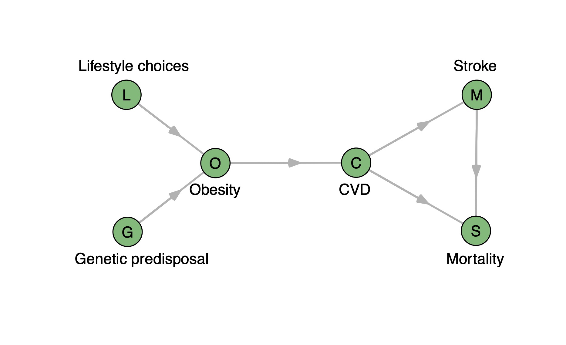
To illustrate the approach and simultaneously a weakness of shna, the following directed graph is introduced (Figure 1). There are two input variables depicted as nodes, genetic predisposal and lifestyle choices, that influence the target variable obesity. Obesity heightens the risk of cardiovascular diseases (CVD), and CVD in turn increases mortality among the affected population. Additionally, CVD is a risk factor for stroke, hence the graph also includes a directed edge from the node CVD to the node stroke. Stroke, on the other hand, greatly increases mortality, whose node ends up as the sink node. Note that the triangle on the right is not a cycle due to the directionality of the edges. Therefore, the resulting network is a typical directed acyclic graph (DAG).

Figure 1  A directed so-called Werner graph visualizing the obesity-mortality example. Nodes represent variables and edges direct interactions between them. CVD: cardiovascular diseases.

Due to its approach to find linear association chains, snha struggles with the detection of ramifications. When given a dataset or correlation matrix based on the example graph, it is most likely to miss one of the outgoing edges from CVD. However, the potentially missing relationship describes a causative relationship, thus it is too important to ignore (and tolerate) its absence. Accordingly, the aim of this study is to improve the capability of snha to detect ramifications in the underlying interdependencies of the input data with only little increase in runtime.

Materials and methods

Software

Programming was done exclusively with the language R for this project (R Core Team 2022). Additionally, the R packages used include huge (Jiang et al. 2021), qgraph (Epskamp et al. 2012), ergm (Krivitsky et al. 2023), snha (Groth 2023), mcgraph and asg (Groth 2022), of which huge, qgraph and ergm can be considered references of network reconstruction. Synthetic data was generated with functions from the mcgraph package (Novine et al. 2022). A public version of mcgraph can be found within the snha package called mgraph.

Graphs used

Barabasi graphs, also known as Barabasi–Albert (BA) models, are a type of scale-free network characterized by preferential attachment mechanism, where new nodes are more likely to connect to existing nodes with higher degrees (Barabasi and Albert 1999).

Density in the context of graphs refers to the ratio of the number of actual edges in the graph to the maximum possible number of edges among all nodes. It provides a measure of how closely knit the connections are in the network, with higher density indicating more connections per node and lower density signifying fewer connections per node (Diestel 2017).

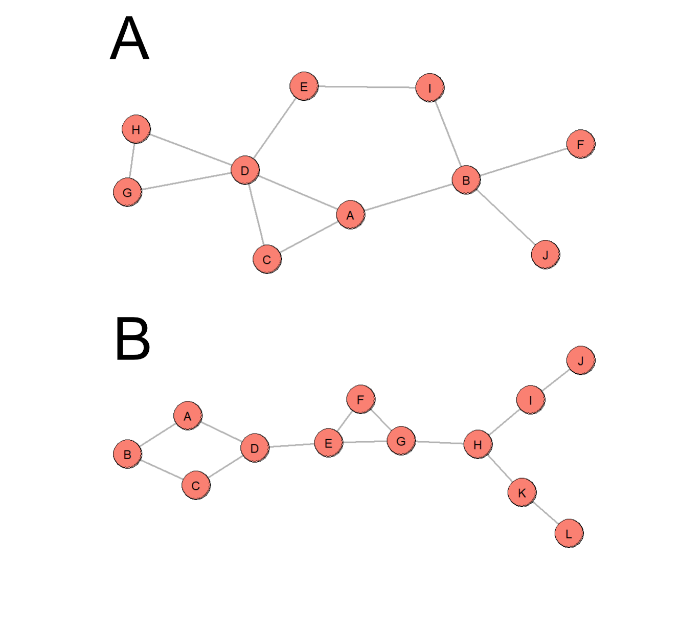
The graphs analyzed include Barabasi graphs (Barabasi and Albert 1999) of density 1.5 denoted as M1.5, Werner (W) and Wernerextended (WX), an extended version of W, graphs. WX has an additional diamond-like structure and a longer branching path compared to W. We included the M1.5 as it was suggested to be a more reasonable representation of biological networks. These M1.5 graphs were made in a way that either adds 1 or 2 edges at each step of the Barabasi graph generation. We chose to only include Barabasi graphs with 20 nodes. The Barabasi graph in Figure 2 has 10 nodes and WX is shown with 12 nodes as visual representations of the graphs used in our tests.

Figure 2  A: Barabasi graph with 10 nodes of densities 1.5 B: Wernerextended graph with 12 nodes.

Data generation and benchmarking

In order to benchmark different graph prediction methods, we decided to create synthetic data using Novine’s Monte Carlo implementation (Novine et al. 2022), the function is called mgraph.graph2data from the public snha package. Some testing was done with huge data generation. Synthetic data built upon a known graph that we gave as an input allows us to easily compare the predicted graph against the original one.

The huge package contains implementations of different methods for network reconstruction, of which we chose correlation thresholding (ct), Meinshausen-Bühlmann (mb) (Meinshausen and Bühlmann 2006) covariance selection and graphical least absolute shrinkage and selection operator (glasso) (Friedman et al. 2008). As in most cases the true underlying graph structure is unknown, we opted to use the automatic lambda selection function for the huge methods. Furthermore, glasso and lasso implementations of qgraph were chosen with either Bayesian Information Criterion (bic) or extended Bayesian Information Criterion (ebic) (Epskamp et al. 2012).

To complement these approaches and provide a comparative methodological framework, we incorporated Exponential Random Graph Models (ergm) from the ergm package (Krivitsky et al. 2023). The ergms are particularly well-suited for modeling complex network data through specified probability distributions over graphs, thus offering a robust alternative to regularized regression techniques used in glasso and lasso (Krivitsky et al. 2023). This allows us to contrast the performance of traditional regression-based network reconstruction techniques with that of stochastic models tailored for social network analysis and other fields where the underlying network dynamics are inherently probabilistic.

The benchmarking procedure was generally structured as follows: Initially, a graph was constructed utilizing the mgraph.new function from the asg or the snha package. The adjacency matrix derived from this graph served as a blueprint for the generation of simulated data. This simulation aimed to mimic real data as accurately as possible by maintaining the graph’s interdependencies in a balanced manner and incorporating random noise, ensuring that the inherent connections were neither exaggerated nor understated (Novine et al. 2022). The result was a synthetic dataset wherein the quantity of variables matched the number of nodes in the graph. This dataset, or its correlation matrix if necessary, was then used as input for the graph estimation functions, which produced the adjacency matrix of the estimated graph. The final step involved evaluating each method’s performance by contrasting the estimated graph with the original one.

Accuracy metrics used

There has long been disagreement in the scientific community about which accuracy standards should be used (Bekkar et al. 2013), most of these metrics are based on ratios of true positives (TP), true negatives (TN), false positives (FP) and false negatives (FN). In our case, they correspond to correct and incorrect numbers of predicted edges or non-edges.

The sensitivity (Sens) is defined as the ratio of true positives to the sum of true positives and false negatives.

The specificity (Spec) is defined as the ratio of true negatives to the sum of true negatives and false positives.

Precision (Prec) is calculated as the ratio of true positives to the sum of the true positives and false positives.

The Matthews Correlation Coefficient (MCC) (Chicco and Jurman 2020) is calculated as follows:

As the MCC does not fully capture the disproportionate gain of either Sens or Spec compared to the other, we included the Balanced Classification Rate (BCR) (García et al. 2009) and No Information Rate (NIR) (Bicego and Mensi 2023). BCR is the average of Sens and Spec, so a large gain in Sens with a small loss in Spec will still yield a better BCR.

One could say that NIR is something like an estimate of the most common class without any information and serves as a baseline metric. If for example 70% of the data is class A and 30% is class B, then estimates of class A would every time yield an accuracy of 70%. The NIR, in this context, represents this baseline accuracy. Therefore, the NIR is used to compare model accuracy against a baseline. If the accuracy (Acc) surpasses the NIR greatly, it has significant predictive power. Therefore, Acc and NIR should be viewed together. The Acc is calculated as the ratio of the sum of true positives and true negatives to the total number of cases.

R squared gaining

The extension called R-squared gaining (rsg) follows the concept of aiming at improving a specific scoring measure. In rsg, the aim is to maximize the gain in adjusted R-squared values obtained with the lm function in the stats package of base R. The R-squared value represents the proportion of variance of the response variable, here the target node, that is explained by the predictor variable(s), or the source node(s). The normal R-squared statistic refers to the sample and the adjusted R-squared value to an estimate in the population (Miles 2005).

For every node i in the graph, rsg searches for candidate nodes with which a new edge appears meaningful, with respect to their original correlation coefficients and p-values, which are output by default snha. Then, a linear regression model was fitted with the node i as response variable and the already connected node(s) as predictor variable(s). A second model included the candidate node as additional predictor variable. If the second model resulted in an adjusted R-squared value higher than the first model, and if the difference was over a specified threshold, then the edge between the node i and the candidate node was added to the graph. This threshold was the only parameter in this extension and consequently, it was tested for a range of values.

Linear model check

Another method, linear model check (lmc), has been implemented for this project. After obtaining a predicted graph, for example via the default snha, using linear models to check the obtained snha graph to the data, edges will be removed by lmc if they do not add more than a set threshold of the adjusted R-squared value. We set the default threshold to two percent.

Combinations

The novel approach in this project was the combination of extensions of snha, as weaknesses and strengths of each method may balance each other out.

Multiple combinations of extensions were tested. A combination of rsg and lmc was thus denoted as rsg_lmc, which initially applied rsg followed by lmc and lmc_rsg follows the same naming-logic in inversed order, meaning that we first applied lmc and then rsg. That means that lmb combined lmc and bootstrapping (boot) and boot_lmc_rsg combined boot, lmc and rsg.

Afterwards, pairwise t-tests were conducted to compare whether the extensions significantly outperformed or underperformed compared to the default snha. These t-tests were performed in a paired manner with each individually created graph at each run. This enhanced the comparability as a particularly poor prediction on a “harder graph”, e.g. containing diamond and triangle patterns, which are more challenging to resolve, will not be compared against a good prediction of a different method on an “easy graph”. Due to the nature of the Barabasi graph generation, some randomness can be expected, which enabled the possibility of creating graphs of varying difficulty in regard to the ramifications.

Results

Overview

Interestingly using huge data generation yielded better results for the methods from the huge package. Both ct and mb benefited heavily from using the synthetic data generated by the huge function, whereas performance was worse when using our generated data. All other methods did not show this trend, thus we decided to only include results using Novine’s MC data generation (Novine et al. 2022).

The new extensions yielded better results, especially combinations of rsg and lmc in either orientation. Using both subsequently generally produced better results than each method in isolation when regarding the MCC. Compared to the reference methods of the huge, qgraph and ergm packages, our methods seem to consistently strike a better balance between Sens and Spec, since neither of those two metrics dips below 0.5 for any combination of snha extensions. 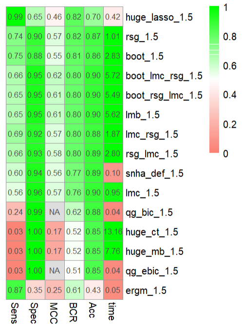A comprehensive overview can be seen in Figure 3.

Figure 3  Heatmap showing the means of 10 runs of M1.5 with 20 nodes for Sensitivity (Sens), Specificity (Spec), Matthews correlation coefficient (MCC), Balanced Classification rate (BCR), time in seconds and accuracy (Acc) for network reconstruction methods huge correlation threshold (huge_ct), huge lasso (huge_lasso), huge Meinshausen-Bühlmann (huge_mb) , qgraph glasso with bic (qg_bic), qgraph glasso with ebic (qg_ebic), exponential random graph models (ergm), St. Nicolas House Analysis (snha) and its extensions Linear Model Check(lmc), R-squared Gaining(rsg) and bootstrapping (boot).The Null Information Rate (NIR) to compare against is 0.85.

Matthews correlation coefficient and balanced classification rate

Barabasi M1.5

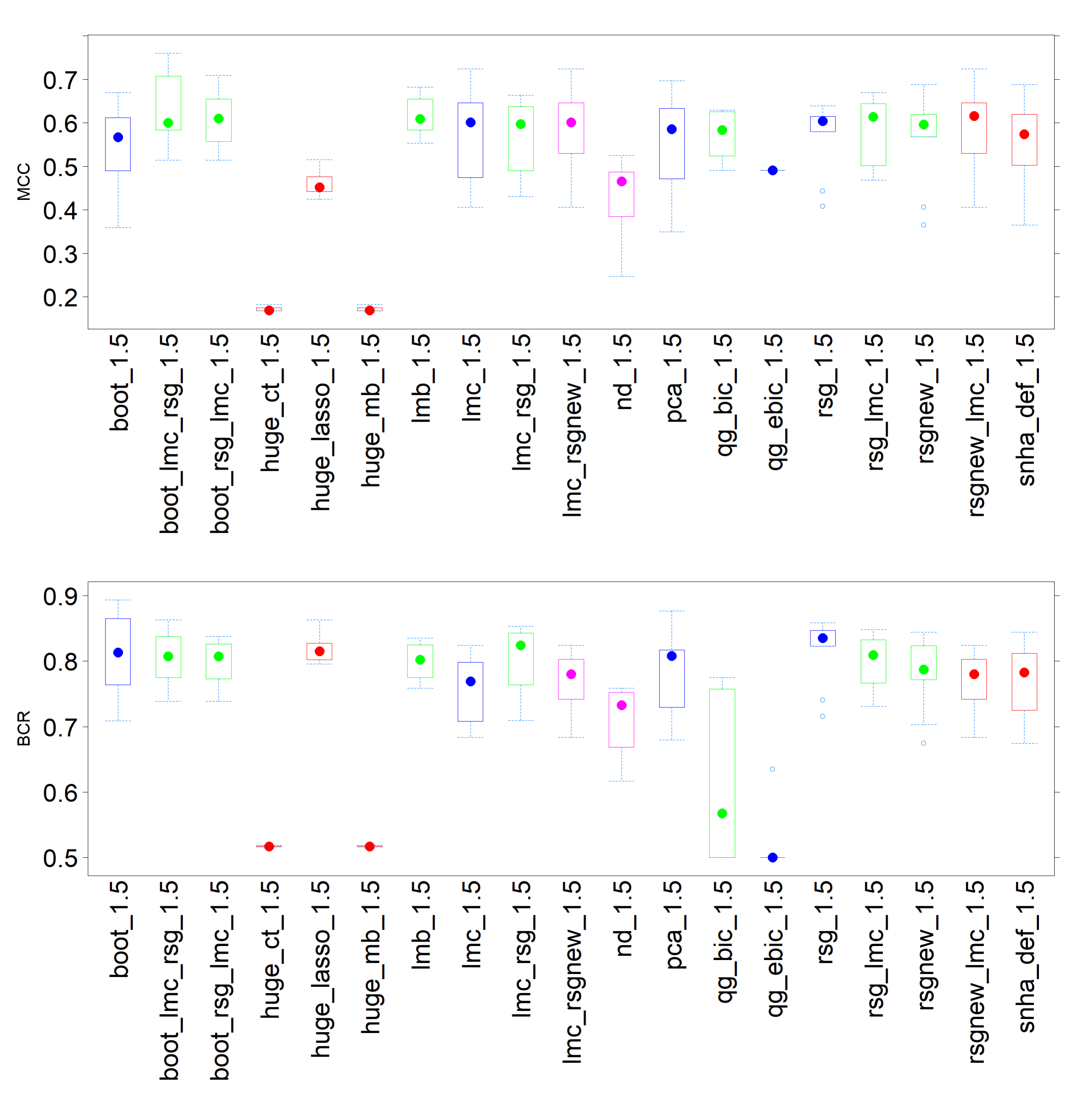
Figure 4 shows a box and whiskers plot for the MCC and the BCR. Within the scope of MCC, it is observed that the boxes are generally quite elongated for all methods. This observation implies a lack of consistency across the performance of all methods.

When considering the BCR, the subpar performance of the huge methods, specifically mb and ct, becomes apparent. Despite their high Spec, their Sens is low, which results in a diminished BCR. Conversely, the combinations of lmc and rsg, along with boot, emerge as some of the top performers in terms of BCR. This suggests that these combinations are more adept at striking a balance between Sens and Spec. Additionally, as visible in Figure 1, the MCC was not always calculable for qgraph lasso with bic or ebic as selection criterion.

For M1.5, the range was between 0.8 and 0.9. In all cases, the default shna fell short when compared to boot, lmc, rsg, and combinations of these three.

Figure 4  Box and whiskers plot of Matthews correlation coefficient (MCC) and Balanced Classification rate (BCR) for M1.5 using various network reconstruction methods. Different methods are colorcoded as follows: huge functions are red, qgraph functions are magenta, singular extensions of St. Nicolas House Analysis (snha) and default snha are blue and combinations of extensions are green.

The paired t-tests for BCR, presented in Tab. 1, reveal that most combination methods incorporating lmc significantly outperform the default snha. In contrast, qgraph lasso with bic and ebic, as well as huge ct and mb, perform significantly worse than the default snha. It becomes evident that combinations involving at least either boot or lmc tend to perform better than the default snha.

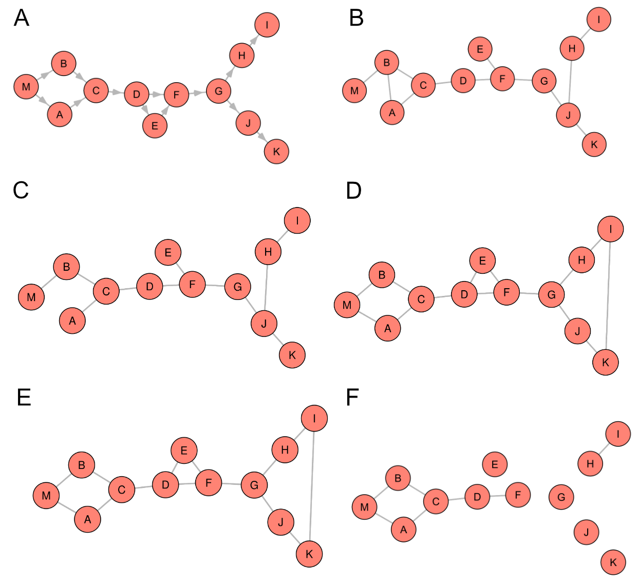
Wernerextended

Figure 5 provides a visual representation of the predicted Wernerextended (WX) graphs using default snha, lmc, lmc_rsg, lmb_rsg and qgraph lasso. The results observed in the Barabasi graphs are mirrored in these graphs. Specifically, qgraph predicts fewer edges, but all of them are correctly identified. In contrast, our methods predict a larger number of edges, some of which are incorrectly predicted. The number of mistakes decreases with the addition of more extensions, but an edge at the end of the branching path between nodes I and K is added for both lmc_rsg and lmb_rsg.

The challenges previously encountered with the triad consisting of nodes D, E, and F have been addressed by the combination of extensions. The branching path originating from node G can also be correctly identified by these combination methods. Interestingly, with bootstrap, lmb_rsg can also reconstruct the diamond-like structure, correctly assigning both edges to nodes A and B from node M.

qgraph, on the other hand, can solve the diamond-like structure and the path from node C to nodes D and F. However, it fails to correctly identify the triad and the branching path.

Figure 5  Applying different graph estimation methods on Wernerextended (WX) graph. A: original WX, B: default St. Nicolas House Analysis (snha), C: Linear Model Check (lmc), D: lmc and R-squared Gaining (rsg), E: Linear Model Check with Bootstrapping (lmb) and rsg, F: qgraph lasso

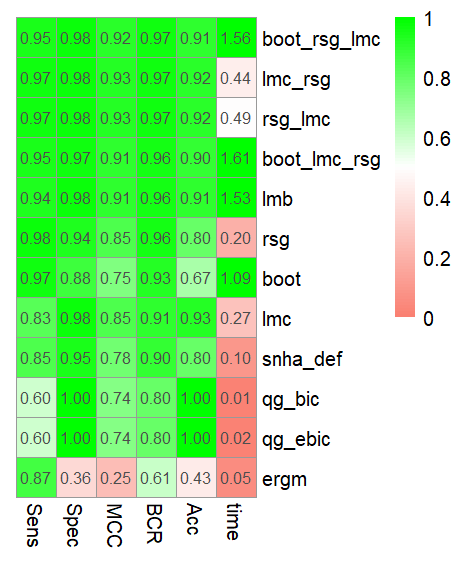
As evident in Figure 6, default snha and qgraph glasso are the least effective at predicting the WX graph based on the BCR and MCC metrics. However, they are the fastest methods in terms of computational time. The combination methods, on the other hand, perform well, with boot_lmc_rsg, lmc_rsg, rsg_lmc and boot_lmc_rsg emerging as the top performers. These methods maintain a high Sens while achieving a very high Spec. While their Spec, at 0.98, is slightly lower than qgraph’s perfect score of 1.00, their Sens, ranging from 0.95 to 0.97, is significantly higher than qgraph lasso’s Sens of 0.6.

The combination methods exhibit better Sens compared to default snha and are close in terms of Spec, indicating that they detected more edges. This observation, in conjunction with Figure 5, confirms that the ramifications that were discovered indeed correspond to the additional edges detected.

Figure 6  Heatmap showing the means of 10 runs of M1.5 with 20 nodes for Sensitivity (Sens), Specificity (Spec), Matthews correlation coefficient (MCC), Balanced Classification rate (BCR),time in seconds and Accuracy (Acc) for network reconstruction methods huge correlation threshold (huge_ct), huge lasso (huge_lasso), huge Meinshausen-Bühlmann (huge_mb) , qgraph glasso with bic (qg_bic), qgraph glasso with ebic (qg_ebic), exponential random graph models (ergm) , St. Nicolas House Analysis (snha) and its extensions Linear Model Check(lmc), R-squared Gaining(rsg) and bootstrapping (boot).The Null Information Rate (NIR) to compare against is 0.80.

Time

All bootstrap variants exhibit a slowdown, with their computational times being at least an order of magnitude greater than the others. The huge methods utilizing the star selection criterion also demonstrate a similar behavior. While rsg_lmc and lmc_rsg perform within an acceptable timeframe, they are noticeably slower than the default snha.

The default snha and singular extensions require a second or less of computational time. Combinations of rsg and lmc take less than 3 seconds, but adding boot to the mix increases the computational time to between 5 and 6 seconds for M1.5.

For M1.5 graphs with 20 nodes, the default snha takes approximately 0.095 seconds, while the boot_lmc_rsg combination requires an average of 5.72 seconds. This equates to nearly a 60-fold difference in computational time.

Discussion

The original intent of snha was to provide a quick overview of one’s data, assisting in hypothesis generation and uncovering intriguing connections between variables. Due to this project and the expansion of extensions for snha, various aspects have changed, such as the computational time requirement.

Given the graph sizes we are dealing with, the additional time investment required for improved results is acceptable. While the computational time might become a concern for larger graph sizes, we anticipate that the number of variables we need to predict will not be so large as to make computational time a significant issue. To put it into perspective, if we were to equate the amount of synthetic data we created for 20 nodes (each with 200 data points) to real-world data, it would be roughly equivalent to the sample sizes in clinical placebo-controlled trials, which typically measure fewer than 20 parameters across several dozens to hundreds of patients, an example would be trials for supplements which typically have less than 50 participants (Wu et al. 2022).

As demonstrated in previous works by Bodenberger (Bodenberger) and Moris (Moris 2023), both bootstrapping and rsg outperform the default snha. Not surprisingly, the combination of bootstrapping with lmc and rsg consistently yielded the best results in Barabasi graphs of varying densities and in the WX graph.

Our results suggest that rsg may be prone to detecting too many edges, as indicated by its high sensitivity and slightly lower specificity. Similarly, some methods have been noted for their propensity to infer a higher number of connections, that may not reflect true biological interactions. For example, Bayesian network approaches are powerful for inferring causal networks but can sometimes result in the construction of overly complex networks, especially when dealing with extensive systems genetics data. The complexity of diseases like Alzheimer’s or type 2 diabetes often requires careful consideration of gene-to-gene and gene-to-environment interactions (Tasaki et al. 2015). Methods developed to simulate co-expression data and evaluate the performance of various network reconstruction models may also exhibit tendencies to generate networks with high edge counts, especially under conditions of varying noise levels and sample sizes. This overestimation can be attributed to the assumptions inherent in the generative models used for simulation and the performance metrics applied to evaluate method outcomes (Tasaki et al. 2015).

Conversely, lmc appears to exhibit the opposite trend. Interestingly, when combined, they seem to balance each other out, while also being faster than any variant of the bootstrap extension.

The less elongated boxes of BCR compared to those of MCC indicate less variability in the BCR scores across different methods. This could suggest that BCR might be a more effective metric overall, providing a more consistent measure of performance across different network reconstruction methods. This consistency could make BCR a more reliable metric for comparing the effectiveness of different methods, particularly when the goal is to achieve a balance between sensitivity and specificity.

“Stability Indicators in Network Reconstruction” discusses the variability of network reconstruction methods which might imply similar observations about the stability and reliability of metrics (Filosi et al. 2014).

In the context of the MCC scores, it is worth noting that the huge lasso method shows a peculiar trend of a slight increase in MCC as the graphs become denser. This could suggest a better performance of huge lasso in denser graphs. This observation aligns with expectations from network reconstruction methodologies, where denser connectivity patterns may provide more data points for lasso-based methods to leverage, potentially leading to more accurate edge prediction. For comprehensive insights into lasso methodologies and their applications in dense graph scenarios, the works by Tibshirani (Tibshirani 1996) on regression shrinkage and selection via the lasso and Meinshausen and Bühlmann (Meinshausen and Bühlmann 2006) on high-dimensional graphs and variable selection with the lasso provide foundational understanding.

Another unique behavior observed only in huge mb, ct, and lasso methods is their tendency to either have a sensitivity or specificity very close to 0 or 1. This indicates that these methods either predict the existence of all possible edges within a given graph or predict a single edge with a high degree of certainty. Chen and Mar (Chen and Mar 2018) bring insight into the sensitivity and specificity trade-offs in network reconstruction and discuss evaluation metrics in the context of gene regulatory network inference. Similar to our testing, Chen and Mar (Chen and Mar 2018) obtained strongly varying networks for different reconstruction methods.

It is notable that the original publications on huge methods may not explicitly discuss the tendency to polarize sensitivity or specificity (Zhao et al. 2020). This gap suggests an opportunity for future research to explore the conditions under which huge methods, particularly in the context of mb, ct, and lasso variants, lean towards these extremes.

Efforts to optimize the current rsg extension have so far resulted in a slight decrease in computational time at the expense of performance. Potential improvements to rsg, aimed at reducing the number of falsely predicted edges, could include changing the current threshold to selection criteria that disproportionately penalize the inclusion of more parameters, such as the Akaike Information Criterion (AIC) (Bozdogan 1987).

5. Conclusion

The inherent ability of the default snha to identify long chains has been preserved in our combination approaches. Therefore, we conclude that our recent combination methods have led to improvements in detecting ramifications and enhancing the overall prediction quality of graphs. This suggests that these combination methods are not only capable of maintaining the strengths of the default snha, but also of addressing its limitations, thereby providing a more comprehensive and accurate network reconstruction.

Acknowledgements

I would like to thank Detlef Groth for his guidance during this project. My sincere thanks also go to Cedríc Morris for his extensive preliminary work which provided a solid foundation for this project. I am grateful to Masiar Novine for stimulating discussions and inspiring ideas. I would also like to thank the International Student Summer School in Gülpe at the University of Potsdam for their support and to the Summerschool KoUP Funding, without which this work would not have been possible. A special thanks goes to Mari Delor who provided me with some data to test our methods.

References

Barabasi, A. L./Albert, R. (1999). Emergence of scaling in random networks. Science 286 (5439), 509–512. https://doi.org/10.1126/science.286.5439.509.

Bekkar, M./Djemaa, H. K./Alitouche, T. A. (2013). Evaluation measures for models assessment over imbalanced data sets. Journal of Information Engineering and Applications 3, 27–38. Available online at https://api.semanticscholar.org/CorpusID:52267786.

Bicego, M./Mensi, A. (2023). Null/No Information Rate (NIR): a statistical test to assess if a classification accuracy is significant for a given problem, 2023. Available online at http://arxiv.org/pdf/2306.06140.

Bodenberger, B. Improved network reconstruction using resampling methods. Project work thesis at University of Potsdam. Potsdam.

Bozdogan, H. (1987). Model selection and Akaike’s Information Criterion (AIC): The general theory and its analytical extensions. Psychometrika 52 (3), 345–370. https://doi.org/10.1007/BF02294361.

Chen, S./Mar, J. C. (2018). Evaluating methods of inferring gene regulatory networks highlights their lack of performance for single cell gene expression data. BMC Bioinformatics 19 (1), 232. https://doi.org/10.1186/s12859-018-2217-z.

Chicco, D./Jurman, G. (2020). The advantages of the Matthews correlation coefficient (MCC) over F1 score and accuracy in binary classification evaluation. BMC Genomics 21 (1), 6. https://doi.org/10.1186/s12864-019-6413-7.

Diestel, R. (2017). Graph theory. 0072-5285. https://doi.org/10.1007/978-3-662-53622-3.

Epskamp, S./Cramer, A. O./Waldorp, L. J./Schmittmann, V. D./Borsboom, D. (2012). qgraph: Network visualizations of relationships in psychometric data. Journal of Statistical Software 48 (4), 1–18.

Filosi, M./Visintainer, R./Riccadonna, S./Jurman, G./Furlanello, C. (2014). Stability indicators in network reconstruction. PLOS ONE 9 (2), 1–24. https://doi.org/10.1371/journal.pone.0089815.

Friedman, J./Hastie, T./Tibshirani, R. (2008). Sparse inverse covariance estimation with the graphical lasso. Biostatistics 9 (3), 432–441. https://doi.org/10.1093/biostatistics/kxm045.

García, V./Mollineda, R. A./Sánchez, J. S. (2009). Index of balanced accuracy: A performance measure for skewed class distributions. In: Helder Araujo/Ana Maria Mendonça/Armando J. Pinho et al. (Eds.). Pattern recognition and image analysis. Berlin, Heidelberg, Springer Berlin Heidelberg, 441–448.

Groth, D. (2022). Asg: Package for generating correlation networks based on association chains. Available online at https://github.com/mittelmark/snha-gui.

Groth, D. (2023). SNHA: Package for generating correlation networks based on association chains. Available online at https://github.com/mittelmark/snha/tree/main.

Groth, D./Scheffler, C./Hermanussen, M. (2019). Body height in stunted Indonesian children depends directly on parental education and not via a nutrition mediated pathway - Evidence from tracing association chains by St. Nicolas House Analysis. Anthropol Anz 76 (5), 445–451. https://doi.org/10.1127/anthranz/2019/1027.

Hemelrijk, C. K. (1990). A matrix partial correlation test used in investigations of reciprocity and other social interaction patterns at group level. Journal of Theoretical Biology 143 (3), 405–420. https://doi.org/10.1016/S0022-5193(05)80036-0.

Hermanussen, M./Aßmann, C./Groth, D. (2021). Chain reversion for detecting associations in interacting variables—St. Nicolas House Analysis. International Journal of Environmental Research and Public Health 18 (4), 1741. Available online at https://www.mdpi.com/1660-4601/18/4/1741.

Huynh-Thu, V. A./Irrthum, A./Wehenkel, L./Geurts, P. (2010). Inferring regulatory networks from expression data using tree-based methods. PLOS ONE 5 (9), 1–10. https://doi.org/10.1371/journal.pone.0012776.

Jiang, H./Fei, X./Liu, R./Roeder, K./Lafferty, J./Wasserman, L./Li, X./Zhao, T. (2021). Huge: High-dimensional undirected graph estimation.

Krivitsky, P. N./Hunter, D. R./Morris, M./Klumb, C. (2023). ergm 4: New features for analyzing exponential-family random graph models. Journal of Statistical Software 105 (6), 1–44. https://doi.org/10.18637/jss.v105.i06.

Logsdon, B. A./Mezey, J. (2010). Gene expression network reconstruction by convex feature selection when incorporating genetic perturbations. PLOS Computational Biology 6 (12), 1–13. https://doi.org/10.1371/journal.pcbi.1001014.

Marks, D. S./Colwell, L. J./Sheridan, R./Hopf, T. A./Pagnani, A./Zecchina, R./Sander, C. (2011). Protein 3D structure computed from evolutionary sequence variation. PLOS ONE 6 (12), 1–20. https://doi.org/10.1371/journal.pone.0028766.

Meinshausen, N./Bühlmann, P. (2006). High-dimensional graphs and variable selection with the Lasso. The Annals of Statistics 34 (3), 1436–1462. https://doi.org/10.1214/009053606000000281.

Miles, J. (2005). R-squared, adjusted R-squared. In: Brian Everitt/David Howell (Eds.). Encyclopedia of statistics in behavioral science. John Wiley & Sons, Ltd.

Moris, C. (2023). Improving ramification detection of St. Nicolas House Analysis. Project work thesis at University of Potsdam.

Novine, M./Mattsson, C. C./Groth, D. (2022). Network reconstruction based on synthetic data generated by a Monte Carlo approach. Human Biology and Public Health 3. https://doi.org/10.52905/hbph2021.3.26.

R Core Team (2022). R: A Language and Environment for Statistical Computing. Vienna, Austria. Available online at https://www.R-project.org/.

Tasaki, S./Sauerwine, B./Hoff, B./Toyoshiba, H./Gaiteri, C./Chaibub Neto, E. (2015). Bayesian network reconstruction using systems genetics data: Comparison of MCMC methods. Genetics 199 (4), 973–989. https://doi.org/10.1534/genetics.114.172619.

Tibshirani, R. (1996). Regression shrinkage and selection via the lasso. Journal of the Royal Statistical Society: Series B (Methodological) 58 (1), 267–288. https://doi.org/10.1111/j.2517-6161.1996.tb02080.x.

Wu, S.-H./Chen, K.-L./Hsu, C./Chen, H.-C./Chen, J.-Y./Yu, S.-Y./Shiu, Y. (2022). Creatine supplementation for muscle growth: A scoping review of randomized clinical trials from 2012 to 2021. Nutrients 14 (6). https://doi.org/10.3390/nu14061255.

Zhao, T./Liu, H./Roeder, K./Lafferty, J./Wasserman, L. (2020). The huge package for high-dimensional undirected graph estimation in R.