Contents

Introduction

A major task in a variety of scientific fields is to identify direct interactions between variables, as this grants insights into their underlying relationship and possibly exposes unwanted effects, for instance in the area of medicine. These interactions can be used to obtain a network representation of the data where edges represent the interaction with nodes, which corresponds to the data variables. Methods such as Lasso- or Ridge-regression heavily rely on the input parameter selection to provide adequate results. Others, like Principal component, factor or cluster analysis are often used to visualize dependencies between the variables in a data set, but they struggle to classify dependent and independent variables. Another recently introduced method is the St. Nicolas house algorithm (SNHA) (Groth et al. 2019; Hermanussen et al. 2021). It is currently available in the R package asg. To attract a wider community, the core functionality of the asg package was reimplemented in Python (van Rossum and Drake 2009). Python was the choice, because it is currently one of the most popular programming languages (University of California 2022; Carbonnelle 2022).

However, methods such as simple correlation or mutual information using simple thresholds fall short of detecting only true direct interactions, as they do not account for indirect or transitive associations between interacting variables. Consider, for example, a gene A directly controls a second gene B, which in turn directly controls a third gene C. Simple correlation would falsely predict a connection between gene A and gene C. Thus, in networks inferred from biological data, with methods such as simple correlation, mutual information, or distance correlation, many erroneous edges would be expected (Marbach et al. 2010; Marbach et al. 2012; Dunn et al. 2008; Burger and Nimwegen 2010; Lapedes et al. 1997). To address this, several methods like partial correlation (La Fuente et al. 2005; Hemelrijk 1990; Veiga et al. 2007) and probabilistic approaches such as maximum entropy model (Lapedes et al. 1997; Marks et al. 2011; Hopf et al. 2012) as well as network deconvolution (Feizi et al. 2013) are used to strengthen direct associations, while removing indirect or transitive ones. These approaches have in common that the result is sensitive to the selection of input parameters.

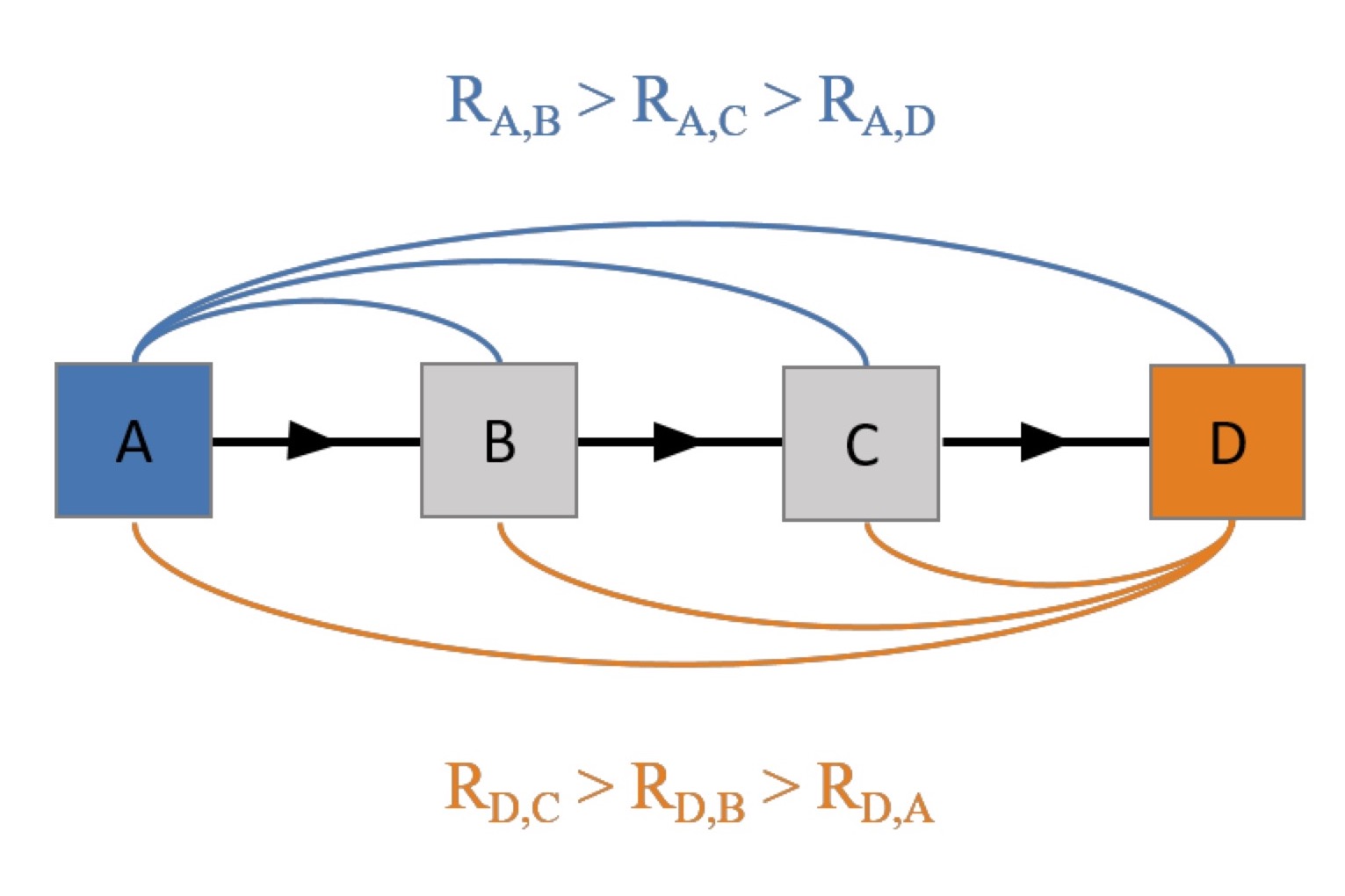
The SNHA (Groth et al. 2019; Hermanussen et al. 2021) is a parameter free approach, which finds direct interactions between variables. The SNHA ranks the absolute correlation coefficients in descending order and thereby creates hierarchic, so called,association chains. Association chains are characterized by sequences for which a reversing start and end point does not change the order of the elements (compare Figure 1). These sequences are used to visualize the dependencies of the underlying variables as a graph by connecting them via undirected edges.

Figure 1  An exemplary association chain with four nodes. It is characterized by the order of pairwise correlation coefficients between the node D and all other nodes, which matches the order of the pairwise correlation coefficients between the A and all other nodes. This ordering builds an association chain and undirected edges connects its members.

Bootstrapping is a method that uses sampling with replacement to provide statistical inferences such as error and bias estimates, confidence intervals, and hypothesis tests without assumptions such as normal distributions or equal variances (Hesterberg 2011). Colby et al. (Colby et al. 2018) have shown that bootstrap aggregation in inferred networks improves stability and, depending on the size of the input data set, it might increases the accuracy. Further, applying bootstrapping to biological networks like gene regulatory networks, can identify high-confidence edges and well-connected hub nodes that potentially play important roles in understanding the underlying biological processes of these networks(Li et al. 2011). The aim of this work is to obtain empirical p-values for predicted edges using the bootstrapping approach, which also stabilizes the prediction quality of the algorithm. Further, testing the algorithm on different graph types will reveal possible limits of the algorithm. And finally, the performance of the SNHA will be compared to the R package asg, to ensure a correct Python port.

Materials and Methods

Software

Major functionalities of the R packages asg (Groth et al. 2019; Hermanussen et al. 2021) and mcgraph (Novine et al. 2022) for the open source software R (R Core Team 2022) were reimplemented using the programming language Python 3 (van Rossum and Drake 2009) (version 3.8.10). Here, the core packages used are pandas (1.3.4), numpy (1.21.3), igraph (0.9.11) and matplotlib (3.4.3). The current R version is available at Groth (2023), while the Python version is available at Hake (2023).

Data

The data used for the analysis was synthetic data for which the underlying graph structure was known. The data was created by the Python implementation of the function mcgraph.graph2data (Novine et al. 2022). It creates data of varying size and density, independent from the graph type using the Monte Carlo method (Metropolis and Ulam 1949), which serves as an input for the SNHA.

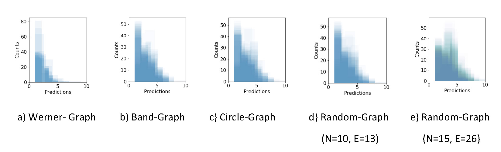
Graph types

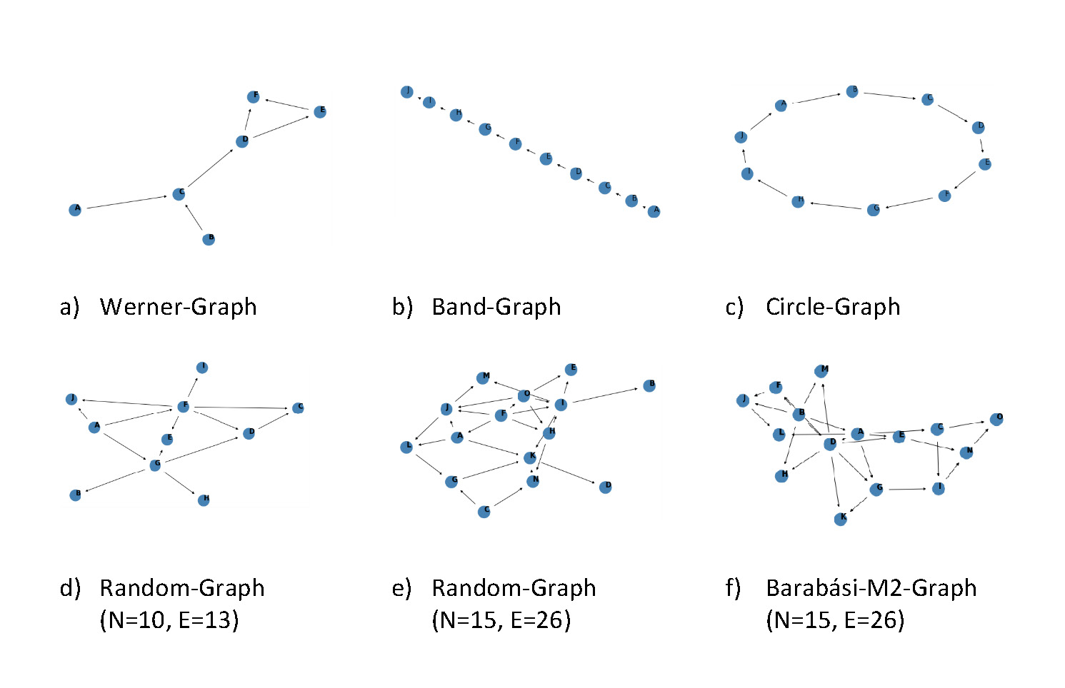
Figure 2  The different graph types used for the analysis.

In the analysis different types of graphs with a diversity in their topology and density were used to get a better understanding in which settings the algorithm performs well and in which not. Examined graph types were Werner-, Hub-, Band-, Circle-, and Random-Graphs (Figure 2).

St. Nicolas house algorithm (SNHA)

The SNHA (Groth et al. 2019; Hermanussen et al. 2021) takes a correlation matrix as its input. In the first step it then loops over the columns of the correlation matrix where each column corresponds to a node in the graph. For each column, the correlations are first ordered according to their absolute values. Then, it looks for association chains by checking if the ordered correlations match forward and backward. If that is the case, a so-called direct chain is found. In case a direct chain was not found in the above step, the algorithm looks for middle chains. In this case, the examined node is placed in all possible positions in the middle of the chain, and it is checked if the resulting sequence of nodes has an ordering of correlation coefficients that matches from forward/backward. After the algorithm has searched for middle chains, the row and the column with the lowest correlated value to the node that is examined at the moment is removed from the correlation matrix and the algorithm continues to search for a direct chain. This procedure is followed until either a chain was found or only 3 nodes remain for the examined chain. After that, the next node is examined. Found chains are then used to establish an undirected graph by establishing undirected edges between the nodes along detected chains.

input data;
procedure Saint_Nicolas_House Analysis (input data);
matrix = correlation(input_data);
for each column of matrix do
	correlation_matrix = matrix
	while length(column) > 3 do
		find longest chain where ordering of correlation 
		matches forward and backward;
		if no chain was found then
			search Middle-Chain;
		end
		remove row and column of correlation matrix with smallest
		correlation coefficient to the column (node) examined at the moment;
	end
end

Quality measure for prediction

The metrics used to evaluate the prediction of the edges based on the correlations is the Balanced Classification Rate (BCR) (Brodersen et al. 2010) and the Matthews correlation coefficient (MCC) (Matthews 1975). These measures result from the counts of true positive (TP), false positive (FP), true negative (TN) and false negative (FN), which are gathered in a confusion matrix. The BCR is defined as:

with

It is used to evaluate binary classification problems. Here, we predict whether two nodes are connected by an edge or not. It is particular useful for imbalanced data, e.g. sparse or dense adjacency matrix, which results in a graph with few edges or a highly connected graph, respectively. The BCR is defined in an interval of [0, 1]. An algorithm that guesses randomly should have a BCR value of around 0.5 or slightly higher. For example, predicting all possible edges as existing would have a sensitivity of 1, but a low specificity if the number of real edges is low in comparison to the total number of possible edges. The MCC is defined as:

The MCC is defined in the interval of [−1, 1], so random guesses lead to values around zero,while solely false predictions produce values down to -1 and solely true predictions cause values of 1.

Empirical p-values by bootstrapping

The empirical p-values (Davison and Hinkley 1997) were calculated with the bootstrapping approach that was applied to the synthetic data produced for the graph types described above. Therefore, a randomized dataset is created by taking k samples (with replacement) from the synthetic data and shuffle it column wise. Afterwards, the edges are predicted by the SNHA. This procedure is repeated m-times and the number of predictions per edge is counted. Repeating this procedure n-times leads to a distribution for each edge, which is used to compute the p-value. Also, the SNHA predicts the edges on the synthetic data m times and sums the number of predictions per edge. The p-value is calculated by North (North et al. 2003):

r is the number of predictions of the randomized data, which is equal or greater than the number of predictions of the synthetic data. While n is the number of repetitions described above. On the other hand, the upper boundary of the confidence interval of the distribution yields a significance threshold for the number of predictions.

Results

After the implementation of the SNHA in Python it was compared to the original R package. Therefore, the graphs from above where used to generate synthetic data (Novine et al. 2022). This data was passed into the R and Python packages to predict the networks. Both implementations of the algorithm yield the same graph predictions. However, the bootstrapping routine leads to slight differences as they depend on the resampling of the data.

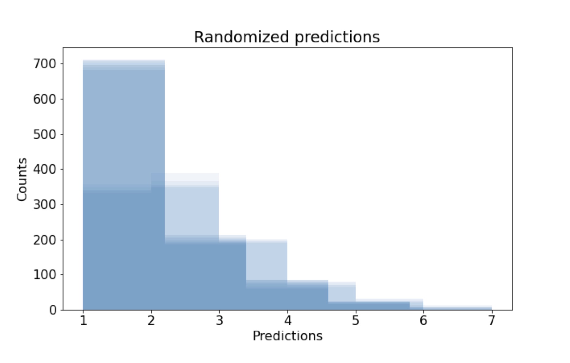
The computation of the empirical p-values (Davison and Hinkley 1997) via bootstrapping demands predictions on randomized data. As a test case, the Werner graph (Fig. 2a) with 1000 iterations and 100 sampling trials per iteration was used to count the random predictions for each edge (Fig. 3). Further, the prediction on the synthetic data without randomization is needed to compute the empirical p-value (Eq. 1).

Figure 3  The distribution of all edge predictions after a column wise randomization of the Werner graph. 1000 iterations with 100 sampling trials per iteration are used to count the number of predictions. On the x-axis the number of predictions in a single iteration (e.g., the bar height of around 100 at 4 predictions means, that in 100/1000 iterations an edge was predicted 4 times during the 100 sampling trails).

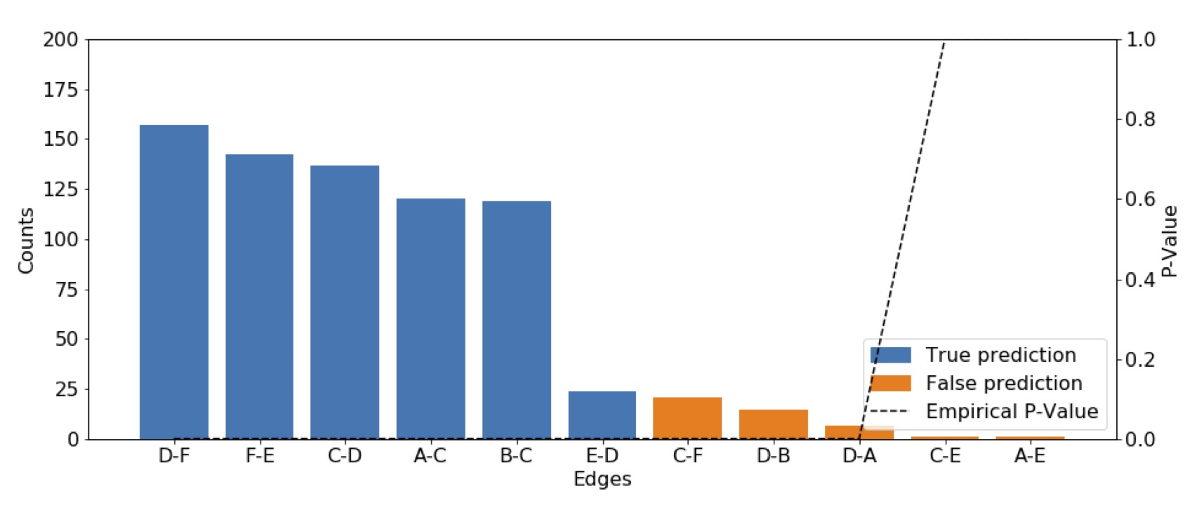
Figure 4 shows the prediction on the synthetic data. The blue bars represent the cumulative count of the true predictions, while the orange bars account for the false predictions in the Werner graph (Fig. 2a). Next to the number of predictions the empirical p-value for each edge is plotted, which is below the significance threshold of 0.05 for the edges D-F, F-E, C-D, A-C, B-C, D-E, C-F, D-B, and D-A (Fig. 2 a).

As the number of predictions drops towards one the p-value grows to one. In order to reduce the computational effort to compute the empirical p-values, assume the randomized predictions are binomial distributed. Then the p-value computation reduces from the multiple prediction of random data to a binomial test with a certain probability of success. The test statistic z on the null hypothesis is the following:

and

with

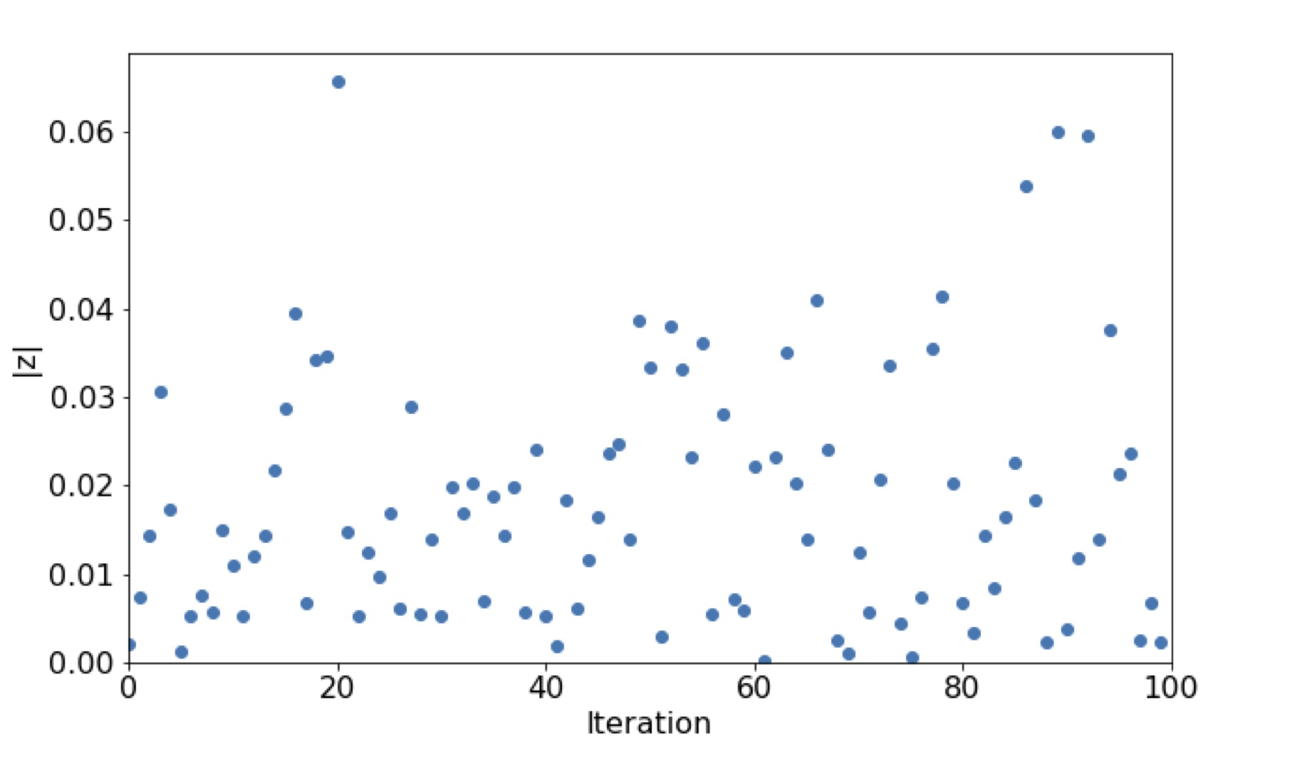
$\widehat{p_1}$ is the probability of success proposed by the distribution of predictions on the random data, $\widehat{p_2}$ is computed by sampling from a binomial distribution $B(n_1,\widehat{p_1})$and n₁ = n₂ = 1000 are the number of iterations. The null hypothesis will be rejected if |z| > 1.65, which is the critical value for a right sided z-test (the limitations for the test are discussed later). Figure 5 shows 100 repetitions for the z calculation for the proposed $\widehat{p_1}$ computed from the distribution in figure 3. The null hypothesis holds true (Fig. 5), so the distribution of the predictions on the randomized data follows the binomial distribution with a success probability of $\widehat{p_1}$.

Figure 4  Cumulative predictions of undirected edges in the Werner graph on 100 samples. The true predictions are plotted in blue, while the false predictions are plotted in orange. The predictions are undirected so the maximum appearance of an edge is 200. The black dotted line is the empirical p-value (e.g., for the edge C-E the p-value is 1.0).

Figure 5  The absolute value of the right sided z-test statistic. The null hypothesis H0: p1 = p2 will be rejected if |z| > 1.65 (Eq. 2). p1 is the probability of success estimated from the distribution shown in figure 3, while p2 is estimated by sampling from a binomial distribution $\mathit{B}\left({\mathit{n}}_{\mathbf{1}},\widehat{{\mathit{p}}_{\mathbf{1}}}\right)$, with n₁=1000.

After showing for the test case that the distribution in figure 3 follows a binomial distribution, it can be assumed that the distributions of the predictions on randomized data for the other graph types also follow a binomial distribution (Fig. 8 supplement material). Now, the interest shifts to the probability of success, as the binomial test needs this probability as an input. Here, success represents finding an edge.

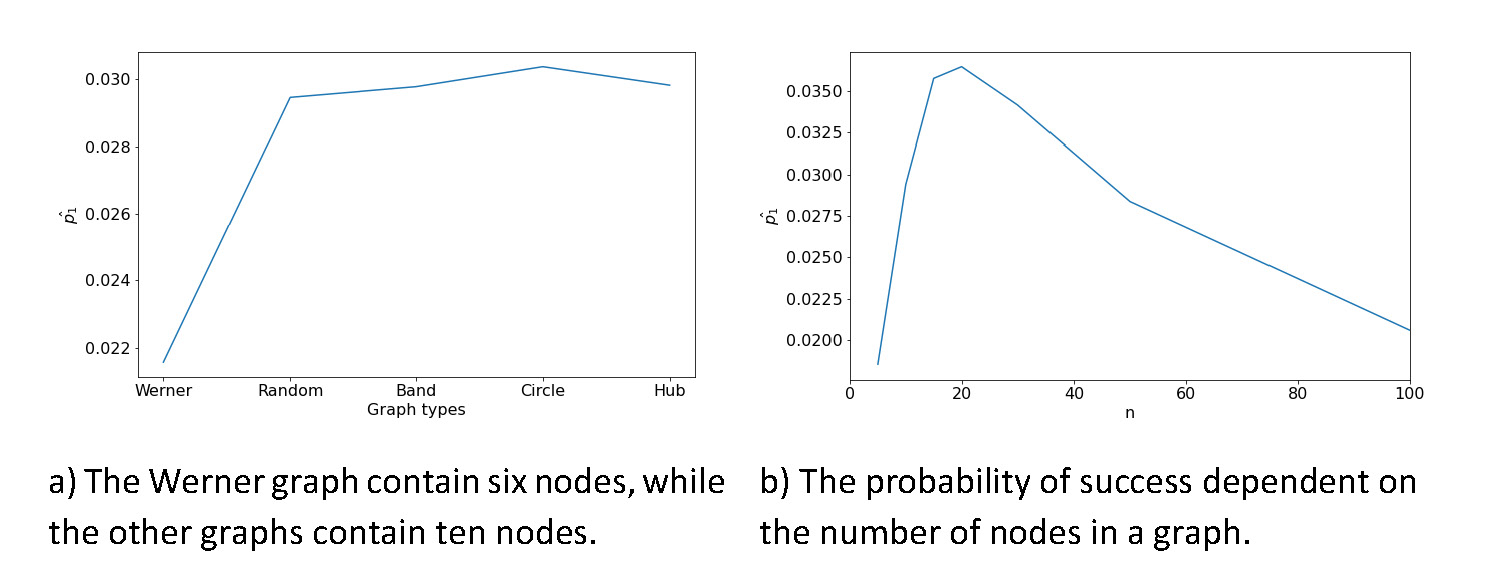
Figure 6  Influences on the probability of success, which is the likelihood of predicting an edge. These probabilities result from the randomized data for the different graphs (compare Fig. 8 and Eq.1).

The probability of success resulting from the distributions of the other graph types is shown in figure 6a. The probability of success is lowest for the Werner graph and stays constant afterwards. The main differences between the Werner graph and the other graph types are the number of nodes. The Werner graph has six nodes, while the other graphs in this comparison contain ten nodes. The driving factor for the probability of success seems to be the number of nodes in a graph. To predict the probability of success based on the number of nodes, different random graphs with 5, 10, 15, 20, 30, 50 and 100 nodes were created to compute the probability of success (Fig. 6b). After showing that the randomized data is distributed binomially and estimating the probability of success $\widehat{p}$ (Fig. 6b), the p-values can be computed by the binomial test. For example, using the bootstrap settings of λ = 0.20 and n = 20 yields a p-value ≤ 0.004 for all edges found (using $\widehat{p}=0.035$; Fig. 6b). In general, the p-values for all edge predictions can be computed by the binomial test. Using this test to compute the p-values reduces the computational effort, because the number of iterations within the bootstrap routine are reduced and the computed p-values are still reliable.

In order to compare the algorithm with and without using bootstrap 20 random graphs (N=20, E=35 & N=20, E=60) were created. The algorithm predicts the network on the correlation data with and without using bootstrap (Fig. 7). For this test the number of iterations within the bootstrap routine is 30 (n=30) and the threshold for an edge to be accepted as a prediction is 20% (λ = 0.20). In general, the statistics are similar comparing the prediction with and without bootstrap. However, using the algorithm with bootstrap increases the sensitivity, BCR and MCC, especially in the case of higher edge density (see also Tab. 1). The specificity does not increase, nor decrease using the SNHA with bootstrap. As the edge density increases, the overall performance is reduced, but the specificity stays close to 1.00. The speed of the algorithm was tested on a graph with 100 nodes. It runs 1.2s $\pm$ 14.9ms without bootstrapping (measured using timeit cell magic in Jupyter Notebook). While the bootstrap routine increases the runtime by a factor of about 10n (n is the number of bootstrap iterations).

Finally, the random graphs here shown were compared to the Barabási-M1 and -M2 graphs (Barabási and Albert 1999), as these graphs are representative for networks occurring in social and biological processes. Here again, 20 graphs each are created and predicted using the SNHA with and without bootstrap. The table 1 shows that the algorithms prediction on the proposed random graph and Barabási graphs are similar. Also, the difference between using the algorithm with bootstrap and without bootstrap behaves equally for the different graph types.

Discussion

The SNHA is a robust, non-linear and parameter free visualization method for multivariate data. It was developed recently and verified in a few studies (Groth et al. 2019; Dorjee et al. 2021; Hermanussen et al. 2021; Scheffler et al. 2021). It displays associations between variables in a graph yielding immediate insights into the principle data structure. The SNHA assesses variable chains from three up to ten nodes, which allows an understanding of large-scale interactions between the variables. The search for tools to reconstruct networks based on correlations led to code snippets to identify edges. However, these examples (Yan Holtz 2018; Cortez 2017) do not go beyond pairwise comparisons of correlations. Since the code was only available in a R package,its use was limited to researchers comfortable in this programming language, so, it was ported to Python. The Python port yields the same results for the same data sets as the R asg package.

The empirical p-value computation and the binomial test suggest that all edge predictions occurring in 7% of the bootstrap iterations are statistically significant. Next, the p-value computation is discussed in more detail. The significance of the found edges are computed both empirically and by the binomial test. In order to be statistically sound, the predictions on randomized data needs to be binomial distributed. To test for binomial distribution the right sided z-test was conducted, which is valid if $\widehat{p_1}{n}_1>5$ and $\left(1-\widehat{p_1}\right)n_1>5,$ and similarly for $\widehat{p_2}$ and n_2. On the low probability of success (Fig. 6b) and a n = 100, the condition $\widehat{p_1}{n}_1$> 5 is not met. However, the empirical p-values as well as the binomial test suggeststhat an edge becomes significant if it is predicted six out of 100 times with the bootstrap routine. Selecting all significant edges as predictions would increase the false positive predictions. The restrictive parameter λ acts as a threshold for the number of appearances of an edge within the bootstrap routine (e.g., λ = 0.5 means an edge needs to be found in 50% of all bootstrap iterations to be accepted as a predicted edge). The impact of the threshold on the network predictions is shown in the supplement material (Fig. 9). It is unlikely to find an association chain randomly, as the probability of success estimations from the distribution of number of edge predictions on randomized data yields $\widehat{p_1}<0.04$. In a real-world example one could not find the optimal λ-value, as the underlying network structure is not known. So, to only interpret highly significant edges, a λ ≥ 0.20 might be reasonable, even though the condition of the z-test does not hold.

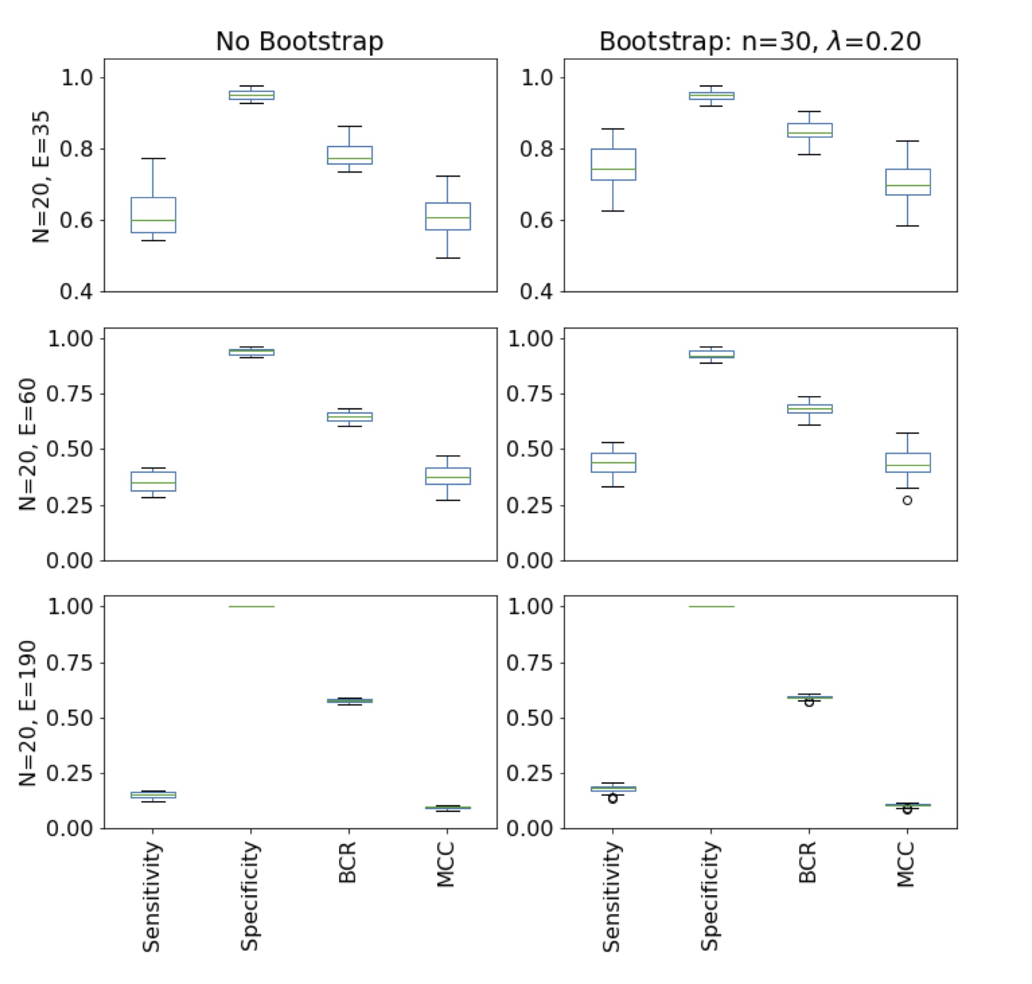
Figure 7  Comparison between the normal St. Nicolas house algorithm used with and without bootstrap. The statistics are computed with the prediction of 20 different random graphs with 20 nodes and 35/60/190 edges each. The bootstrap accepts edges as a prediction if an edge occurs 20% of the iterations (n=30). On one hand, the prediction gets worse as the edge density increases. On the other hand, when using the algorithm with bootstrap the prediction improves.

The predictive power of the algorithm with and without bootstrap was assessed by the metrics sensitivity, specificity, BCR, and MCC on graphs with 20 nodes and a different number of edges (Fig. 7). In general, the evaluation scores decreases as the number of edges increases,while at low edge densities the algorithm performs well. First, the edges found with the algorithm are real edges, as the specificity are in all cases is close to 1.00. Second, the algorithm is better than random guessing as the BCR > 0.5 and the MCC > 0 for all tested graph-types and edge densities. In fact, for graphs with 20 nodes and 35 edges or less it performs very well, as the statistics reaches close to 1.00 (Tab. 1, Fig. 9 in supplement material) for small graphs. Even though the bootsrap approach maintains the pattern of reducing evaluation scores, it improves the prediction (Fig. 7, Tab. 1). However, the slight improvement might not justify the increase in time needed to use the bootstrap approach, as it repeats the algorithm n times. The largest increase is measured in the sensitivity. As the sensitivity increases, while the high specificity stays constant, the BCR and MCC also increase. The algorithm looks for chains and it only finds those which are distinct in correlation. Especially, those chains which contain branches will not be mapped completely, but only one branch will be found. The bootstrap routine helps to identify the branches of the chains as well. By sampling the data set in some cases one branch will be more distinct, while the other branch is emphasized in another case. So, the bootstrap routine identifies further edges which increases the true positive rate. Applying the algorithm on the Barabási-M1 and -M2 yields similar results as the predictions on the random graph proposed above. Therefore, these tests enhance the described results even further. However, the performance is slightly better on the Barabási graphs, because these graphs start with only one controlling nodewhile the random graphs described above contain two controlling nodes, from which the directed graph is built. The controlling points might interfere with each other as the paths converge into a single node. This interference reduces the degree of distinction in correlation, which complicates the extraction of association chains.

Conclusion

The SNHA performs well on the tested graph types, especially on low edge densities. For higher edge densities the prediction can also be improved using the bootstrap routine. The predicted edges are statistically significant. The SNHA (Groth et al. 2019; Hermanussen et al. 2021) was successfully ported from the R package asg to Python (Hake 2023). Both packages yield the same network predictions for the same data sets. Now the SNHA is available in R and Python with direct access to the algorithm for researchers comfortable with these programming languages. Since there is no other tool that goes beyond comparing pairwise correlations, the SNHA could be an enrichment for certain parts of the Python community.

Appendix

Supplement material

Figure 8  The distribution of all edge predictions after a column wise randomization of the Werner graph. 100 iterations with 100 sampling trials per iteration are used to count the number of predictions. On the x-axis the number of predictions in a single iteration is shown.

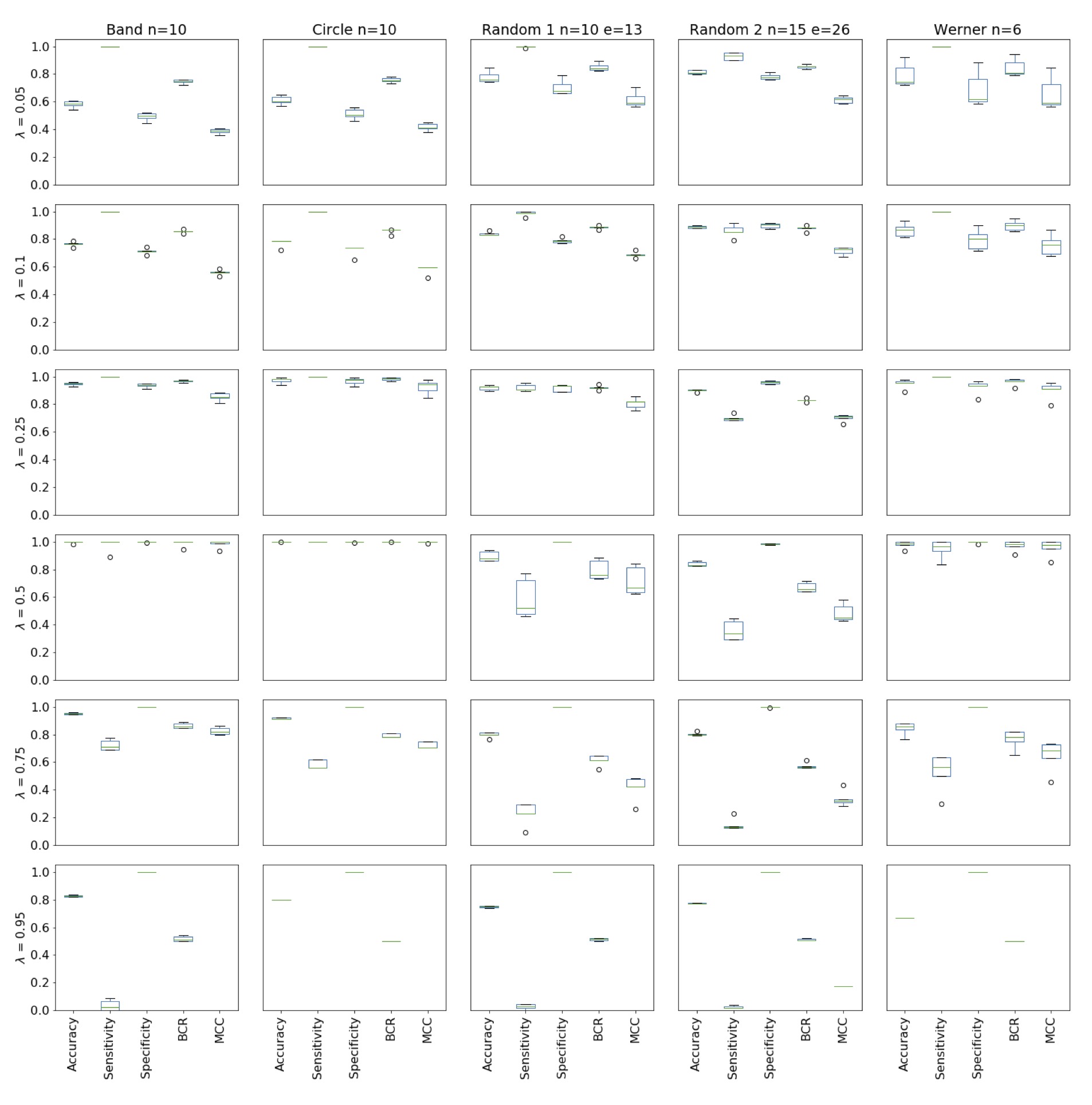
Figure 9  The influence of the λ threshold on the prediction value of the St. Nicolas house algorithm with bootstrap. For each graph five data sets were created. The algorithm predicts each network five times and the mean over the five statistics were computed. Doing it for all five data sets with the corresponding λ threshold leads to the figure above. Choosing λ high (0.75, 0.95) leads to a strong restriction and the predictions are close to a random guess. On the other hand, choosing λ to be low (0.05, 0.10), the false positive number increases and the predictive power becomes low. Also, the edge predictions might not be significant. For the test graph (types Band-, Circle-, and Werner-Graph) a threshold of 0.50 is sufficient to achieve predictions, which are close to the input graph. In order to get high evaluation scores on the random graphs the threshold is 0.25.

Acknowledgements

Special thanks go to PD Dr. Christiane Scheffler and Prof. Dr. Michael Hermanussen for organising the Summer School 2022 on “Human Growth and Development” in Gülpe, Brandenburg. There I had space to start my project, even it is not part of the focus of the Summer School. Further, both of them provided support finishing the project.

References

Barabási, A.-L./Albert, R. (1999). Emergence of Scaling in Random Networks. Science 286 (5439), 509–512. https://doi.org/10.1126/science.286.5439.509.

Brodersen, K. H./Ong, C. S./Stephan, K. E./Buhmann, J. M. (2010). The Balanced Accuracy and Its Posterior Distribution. In: 20th International Conference on Pattern Recognition, 3121–3124.

Burger, L./Nimwegen, E. (2010). Disentangling Direct from Indirect Co-Evolution of Residues in Protein Alignments. PLoS computational biology 6, e1000633. https://doi.org/10.1371/journal.pcbi.1000633.

Carbonnelle, Pierre (2022). PYPL PopularitY of Programming Language 2022. Available online at https://statisticstimes.com/tech/top-computer-languages.php (accessed 12/15/2022).

Colby, S. M./McClure, R. S./Overall, C. C./Renslow, R. S./McDermott, J. E. (2018). Improving network inference algorithms using resampling methods. BMC bioinformatics 19 (1), 376.

Cortez, Valeria (2017). Visualising stocks correlations with Networks 2017. Available online at https://towardsdatascience.com/visualising-stocks-correlations-with-networkx-88f2ee25362e (accessed 12/15/2022).

Davison, A./Hinkley, D. (1997). Bootstrap Methods and Their Application. Journal of the American Statistical Association 94. https://doi.org/10.2307/1271471.

Dorjee, B./Saha, P./Sen, J. (2021). Hierarchy of Associations Between BMI-for-Agez-Scores, Growth and Family Social Status Among Urban Bengali Girls of Siliguri Town, West Bengal: A St. Nicolas House Analysis. Journal of the Anthropological Survey of India 70 (2), 224–239. https://doi.org/10.1177/2277436X211043631.

Dunn, S./Wahl, L. M./Gloor, G. (2008). Mutual Information Without the Influence of Phylogeny or Entropy Dramatically Improves Residue Contact Prediction. Bioinformatics (Oxford, England) 24, 333–340. https://doi.org/10.1093/bioinformatics/btm604.

Feizi, S./Marbach, D./Médard, M./Kellis, M. (2013). Corrigendum: Network deconvolution as a general method to distinguish direct dependencies in networks. Nature biotechnology 33. https://doi.org/10.1038/nbt.2635.

Groth, D. (2023). snha: St. Nicolas House Algorithm for R. R package version 0.1.3. Available online at https://github.com/mittelmark/snha (accessed 7/5/2023).

Groth, D./Scheffler, C./Hermanussen, M. (2019). Body height in stunted Indonesian children depends directly on parental education and not via a nutrition mediated pathway? Evidence from tracing association chains by St. Nicolas House Analysis. Anthropologischer Anzeiger 76 (5), 445–451. https://doi.org/10.1127/anthranz/2019/1027.

Hake, T. (2023). Snha4py: a Python implementation of the St. Nicholas House algorithm. Available online at https://github.com/thake93/snha4py (accessed 2/1/2023).

Hemelrijk, C. (1990). A matrix partial correlation test used in investigations of reciprocity and other social interaction patterns at group level. Journal of Theoretical Biology 143, 405–420. https://doi.org/10.1016/S0022-5193(05)80036-0.

Hermanussen, M./Aßmann, C./Groth, D. (2021). Chain Reversion for Detecting Associations in Interacting Variables—St. Nicolas House Analysis. International Journal of Environmental Research and Public Health 18 (4). https://doi.org/10.3390/ijerph18041741.

Hesterberg, T. (2011). Bootstrap. WIREs Computational Statistics 3 (6), 497–526. https://doi.org/10.1002/wics.182.

Hopf, T./Colwell, L./Sheridan, R./Rost, B./Sander, C./Marks, D. (2012). Three-Dimensional Structures of Membrane Proteins from Genomic Sequencing. Cell 149, 1607–1621. https://doi.org/10.1016/j.cell.2012.04.012.

La Fuente, A. de/Bing, N./Hoeschele, I./Mendes, P. (2005). Discovery of Meaningful Associations in Genomic Data Using Partial Correlation Coefficients. Bioinformatics (Oxford, England) 20, 3565–3574. https://doi.org/10.1093/bioinformatics/bth445.

Lapedes, A./Giraud, B./Liu, L./Stormo, G. (1997). Correlated Mutations in Protein Sequences: Phylogenetic and Structural Effects. Santa Fe Institute, Working Papers 33. https://doi.org/10.1214/lnms/1215455556.

Li, S./Hsu, L./Peng, J./Wang, P. (2011). Bootstrap inference for network construction with an application to a breast cancer microarray study. The Annals of Applied Statistics 7. https://doi.org/10.1214/12-AOAS589.

Marbach, D./Costello, J./Küffner, R./Vega, N./Prill, R./Camacho, D./Allison, K./Aderhold, A./Bonneau, R./Chen, Y./Collins, J./Cordero, F./Crane, M./Dondelinger, F./Drton, M./Esposito, R./Foygel, R./La Fuente, A. de/Gertheiss, J./Zimmer, R. (2012). Wisdom of crowds for robust gene network inference. Nature Methods 9, 796–804. https://doi.org/10.1038/nmeth.2016.

Marbach, D./Prill, R./Schaffter, T./Mattiussi, C./Floreano, D./Stolovitzky, G. (2010). Revealing strengths and weaknesses of methods for gene network inference. Proceedings of the National Academy of Sciences of the United States of America 107, 6286–6291. https://doi.org/10.1073/pnas.0913357107.

Marks, D./Colwell, L./Sheridan, R./Hopf, T./Pagnani, A./Zecchina, R./Sander, C. (2011). Protein 3D Structure Computed from Evolutionary Sequence Variation. PloS one 6, e28766. https://doi.org/10.1371/journal.pone.0028766.

Matthews, B. W. (1975). Comparison of the predicted and observed secondary structure of T4 phage lysozyme. Biochimica et Biophysica Acta (BBA) - Protein Structure 405 (2), 442–451. https://doi.org/10.1016/0005-2795(75)90109-9.

Metropolis, N./Ulam, S. (1949). The Monte Carlo Method. Journal of the American Statistical Association 44 (247), 335–341. Available online at http://www.jstor.org/stable/2280232 (accessed 9/12/2022).

North, B./Curtis, D./Sham, P. (2003). A note on calculation of empirical P values from Monte Carlo procedure. American journal of human genetics 72, 498–499. https://doi.org/10.1086/346173.

Novine, M./Mattsson, C. C./Groth, D. (2022). Network reconstruction based on synthetic data generated by a Monte Carlo approach. Human Biology and Public Health 3. https://doi.org/10.52905/hbph2021.3.26.

R Core Team (2022). R: A Language and Environment for Statistical Computing. Vienna, Austria 2022. Available online at https://www.R-project.org/.

Scheffler, C./Nguyen, T. H./Hermanussen, M. (2021). Vietnamese migrants are as tall as they want to be. Human Biology and Public Health 2. https://doi.org/10.52905/hbph.v2.12.

University of California, Berkeley (2022). 11 Most In-Demand Programming Languages in 2022 2022. Available online at https://bootcamp.berkeley.edu/blog/most-in-demand-programming-languages/ (accessed 12/15/2022).

van Rossum, G./Drake, F. L. (2009). Python 3 Reference Manual. Scotts Valley, CA, CreateSpace.

Veiga, D./Vicente, F./Grivet, M./La Fuente, A. de/Vasconcelos, A. (2007). Genome-wide partial correlation analysis of Escherichia coli microarray data. Genetics and molecular research : GMR 6, 730–742.

Yan Holtz (2018). Network from Correlation Matrix 2018. Available online at https://www.python-graph-gallery.com/327-network-from-correlation-matrix (accessed 12/15/2022).