Contents

Introduction

When it comes to human growth, one might think that there is a plethora of research. And while this might be the case for long-term growth, the analysis of growth measured of short intervals as frequent as weekly or even daily (short-term growth) is still an unusual practise (Hermanussen, 1998). When short periods of time are measured, growth becomes an irregular and chaotic process, comprised of periods of continuous growth, steep changes or even no growth at all (Caino et al., 2004). Characteristic for short-term growth are mini growth spurts, which are described as chaotic series of rapid height changes. In healthy neonates, mini growth spurts occur on average every 4-5 days and can have a mean amplitude of 2 mm (Hermanussen 1998, 2013, p. 11). When looking for small variations and increments, such as mini growth spurts, high precision instruments or frequent measurements are necessary. Daily measurements however require a lot of effort, both for anthropologists and for the subjects. More recently, efforts have been made to make height measurements more practicable and user friendly (Rösler et al., 2022; Schrade and Scheffler, 2013). We propose changepoint analysis as a possible new method to detect growth spurts. Changepoints are abrupt variations in the properties of time series data (Aminikhanghahi and Cook, 2017). In order to find these changepoints, the data is divided into different segments, where each segment has its own characteristics. Differences between segments can be differences in mean, variance, slope, periodicity and many more (Siebert et al., 2021). Due to the nature of our datasets and the characteristics of human growth, the mean height is of particular interest. If a growth spurt has occurred, the assumption is, that there is a shift in the mean height of the subject of selected intervals before and after the growth jump. If that difference is significant enough, it is labelled as a changepoint. While this approach, also known as pattern recognition, is often used in machine learning and forecasting algorithms, it has not been applied to growth analysis (Schroth et al., 2021). To assess the applicability of changepoint analysis on short-term growth data, we performed changepoint analysis on artificial growth data generated by the programming language R. We wanted to test the hypothesis that changepoint analysis is able to detect mini growth spurts.

Samples and Methods

Simulated Data

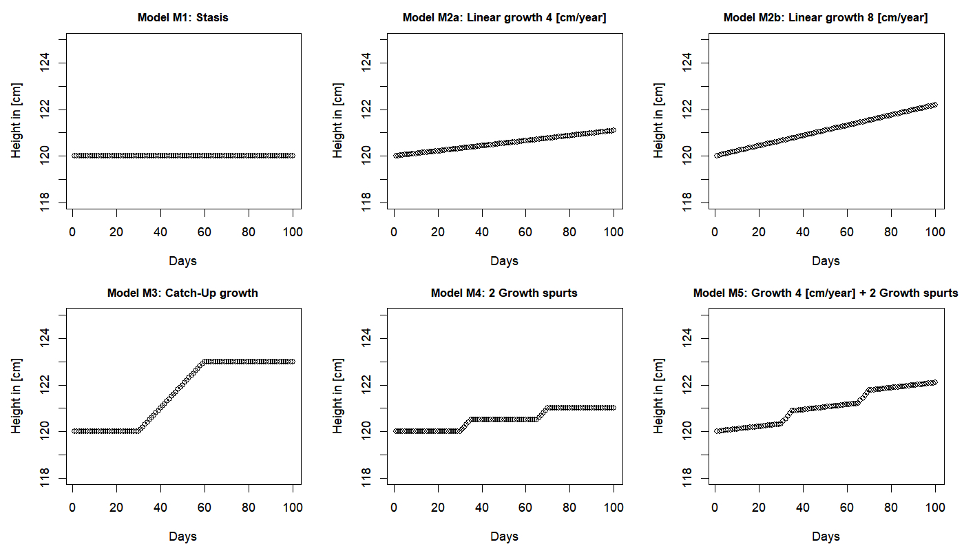
Figure 1  Simulated growth measurements before adding the standard deviation. Each model consists of 100 data points.

In order to validate changepoint analysis for detecting mini growth spurts, six fictional datasets were generated. Based on the descriptions of Caino et al. (2004) and Hermanussen (2013), we created the following simulations (Figure 1):

Models were created using the programming language R. To simulate the measurement error of growth measurements, a standard deviation (SD) was added after the datasets were created. To examine the influence of the SD, different SD values were added to the models. When talking about measurement error, we will refer to different SD added to the models.

Changepoint Analysis

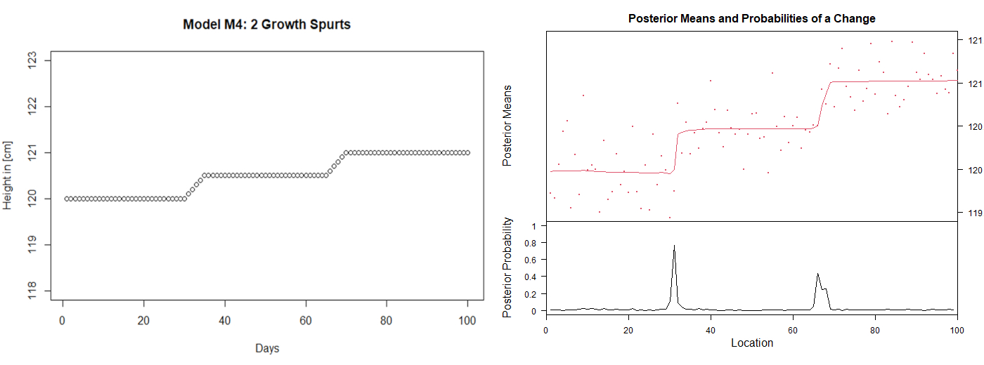
Figure 2  Representative example of changepoint analysis using the bcp package in R. Left: Measurement series of model M4 before SD was added. Two mini growth spurts are visible, starting at day 31 and day 66. Right: The same model after SD was added and changepoint analysis was performed. The red line on the top graph shows an estimation of the posterior mean at each location. An estimate of the probability of a changepoint at any given location is given at the bottom of the graph.

To identify growth spurts we used a Bayesian analysis for changepoints (bcp) proposed by Erdman and Emerson (2007). The bcp package includes an R implementation based on the product partition model proposed by Barry and Hartigan (1993). Using Circular Binary Segmentation (CBS Olshen et al., 2004), bcp estimates the location of change points and splits the time series into different intervals. By looking into the mean of the given interval and comparing it to the neighbouring means an estimation of a changepoint is given. Applied to growth data, the assumption is that, if a growth spurt has occurred, there is a shift in the mean height of the subject between the neighbouring intervals before and after the mini growth spurt. If that difference is significant enough, it is labelled as a changepoint. When plotting the function, bcp gives an estimation of the posterior mean and an estimated probability for a changepoint at any given location (Figure 2). As a non-parametric approach bcp does not need any distribution parameters specified. Another assumption made is, that the used data is stationary. Given that growth is a slow process and mini growth spurts are expected to occur randomly, we expect this violation of stationarity to be neglected.

Rotating and Ranking

In addition to performing changepoint analysis, we were interested if the performance of the algorithm could be improved by preparing the growth data beforehand. By ranking the time series data, we norm the distance of height increments by steps of the magnitude 1. Since height variation due to actual height increments is expected to be much less than height variation due to measurement error, we expected the effect of height increments to be enhanced, while reducing the impact of outliers at the same time. Another approach is to counter the problems that may occur by the data not being stationary. We performed linear regression to estimate a general trend in the time series. By rotating the time series relatively to its mean slope, we repositioned it into a horizontal position. Rotation was achieved using the following rotation matrix which rotates each point of a time series by an angle starting from the origin of the axis. This procedure is rotational invariant, meaning that it does not change the properties of the time series (Bär, 2018; Lin et al., 2012).

Performance Analysis

The output of the algorithm is a “yes” or “no” decision: either there is a changepoint or there is none. Therefore, we reframed the task of changepoint detection as a binary classification problem (Chicco, 2017). By comparing the classification results to the data structure, the algorithm’s performance can be evaluated. In the context of short-term growth, we define the following classifications:

For a given threshold τ, classifier performance was summarised in a contingency table, the Confusion Matrix (CM) (Hoffman et al., 2020). In this study we used the estimated probability of a changepoint as a threshold (Figure 2).

Among the models described in this study, only models M4 and M5 truly contained positive values. The four models M1, M2a, M2b and M3 described growth patterns where no mini-growth spurts occurred. For these models specificity was used to describe the performance as specificity measures the proportion of negative predictions that are truly negative (TNR: true negative rate) (Lalkhen and McCluskey, 2008).

We decided that it is more important for the algorithm to correctly detect growth spurts within reach of their true position than to identify their exact position. Therefore, estimated growth spurts were classified as true positive when they occurred within a distance of plus-minus two days of a true growth spurt. As approximately only 10% of our datapoints represented true positive values, the dataset was imbalanced in favour of negative values. For models M4 and M5 we used the area under the Precision-Recall Curve (PR-AUC) and an averaged and normalised variant of the Matthews correlation coefficient (MCC) (Matthews, 1975) to assess performance. The precision-recall curve captures the relationship between precision and true positive rate (TPR). The TPR, often also referred to as Sensitivity, measures how many of the positive labelled values where TP. Both precision and TPR are concerned with the fraction of TP among prediction outcomes (Novine et al., 2022). This is desirable when the number of positive events is much less than the number of negative ones, i.e. in an imbalanced class distribution. The normalised MCC (norm-MCC) provides a balanced measure even when the classes have different sizes. It produces a high score only if the classifier performs well in all the classes of the confusion matrix (Hoffman et al., 2020). All metrics indicate a perfect classification as the value approaches 1. In most cases, a value of 0.5 indicates a prediction that is not better than random, and a value of 0 indicates total disagreement between predicted and true values. The only exception here being the MCC, which indicated a random classification at 0. Significance between mean differences was determined by performing Welch’s t-test (Bubitzky et al., 2007).

Software

For most of the computations the programming language R (R version 4.1.2) was used. Software packages for additional computations included the bcp package for changepoint analysis (Erdman and Emerson, 2007) and the grid package for the creation of graphs. For the other statistical analyses base R packages were used.

Results

Effect of measurement error on the performance of changepoint analysis

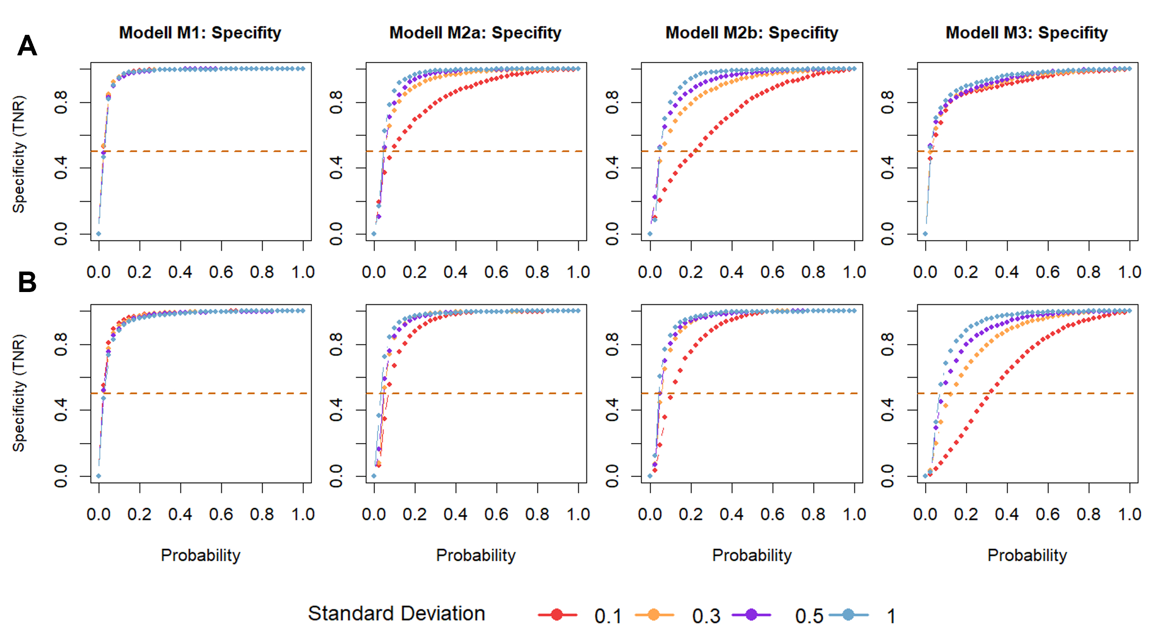
The influence of the measurement error on the algorithm’s ability to correctly identify periods with no growth spurts was assessed by comparing the specificity of changepoint analysis for models M1, M2a, M2b and M3. The algorithm’s specificity increased with increasing measurement error (Figure 3), except for model M1 where no growth occurred at all. In this case measurement specificity was close to 1.

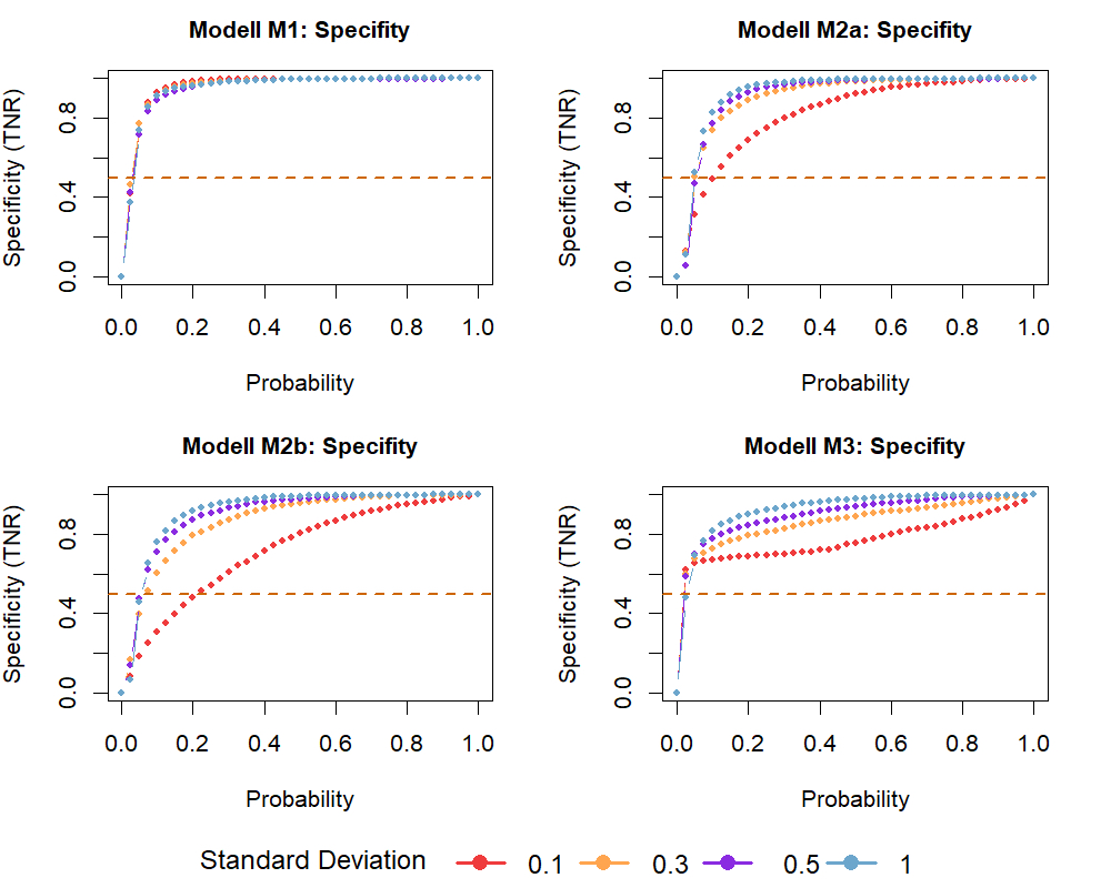
Figure 3  Specificity of changepoint analysis plotted against different probability thresholds. The measurement error is given by the standard deviation (SD). By running 500 iterations for each model and each SD, the influence of the measurement error on the algorithm’s specificity was tested. Models depicted: M1: no growth, M2a & M2b: linear growth and M3: catch-up growth. Dashed lines indicate results for a random classification.

The output of the changepoint algorithm is an estimated probability for a changepoint at any given location (Figure 2). When the probability for a changepoint is used as a cut-off for classification, selecting an appropriate threshold for the probability is important when comparing the metrics. As the probability threshold increases, a higher probability for a changepoint is required for it to be labelled positive, resulting in a higher rate of false negative predictions. When the probability threshold is too low, many changepoints are falsely classified as positive, leading to a higher false positive rate. 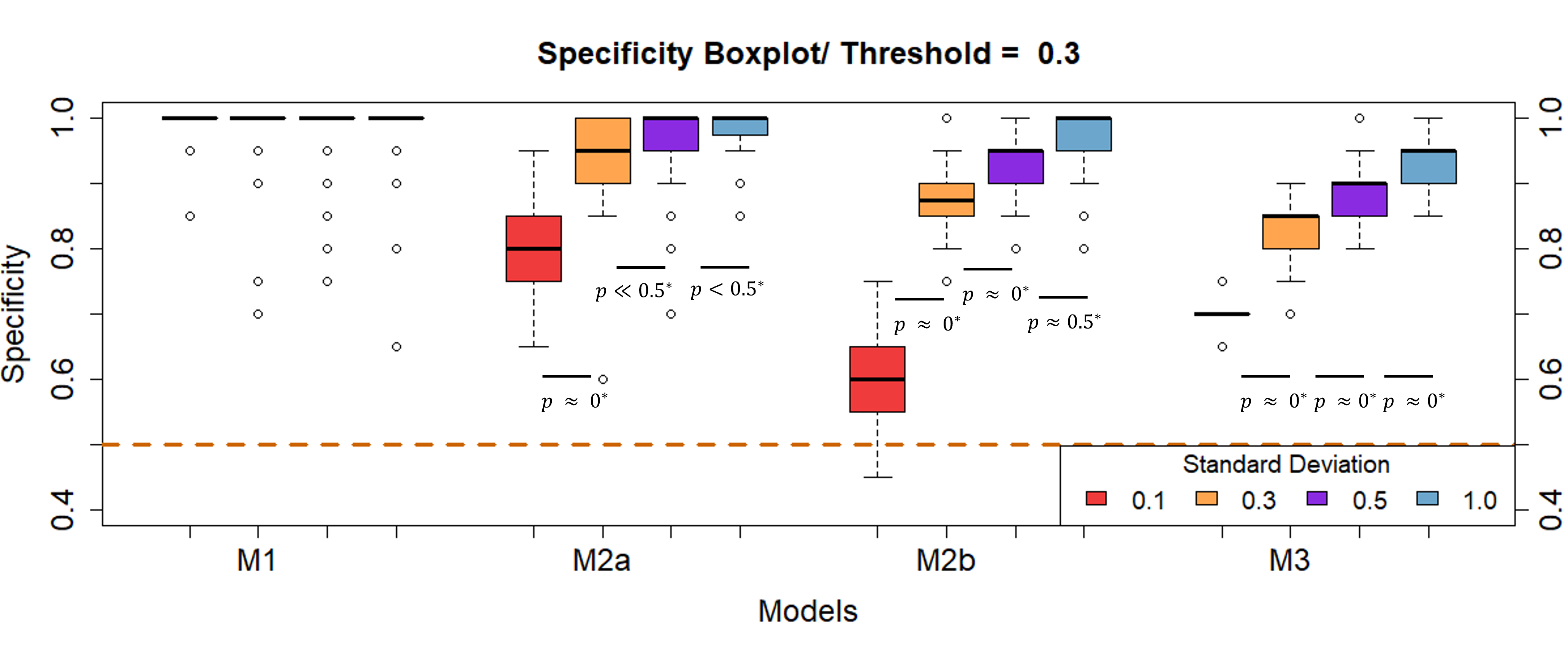We considered a probability threshold of 0.3 a reasonable trade-off between the algorithm’s ability to correctly detect mini growth spurts and to correctly classify growth without growth spurts. Welch’s t-test suggested that there is a significant difference in the algorithm’s specificity for different measurement errors (Figure 4). Mean specificity ranged between 0.8 and 1 for all models except for model M2b that showed a lower specificity of 0.61 for measurement errors around 0.1 cm. Changepoint analysis appears to be able to correctly identify growth periods where no growth spurts have occurred.

Figure 4  Influence of measurement error on the algorithm’s specificity. The measurement error is given by the SD. 500 iterations were performed for each model and each SD. Models depicted: M1: no growth, M2a & M2b: linear growth and M3: catch-up growth. Dashed lines indicate results for a random classification.

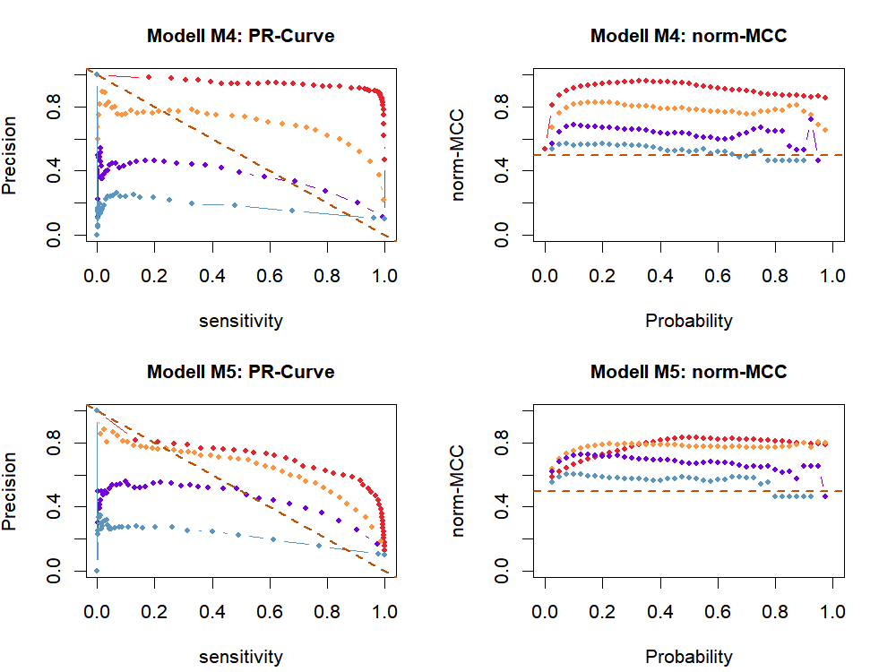
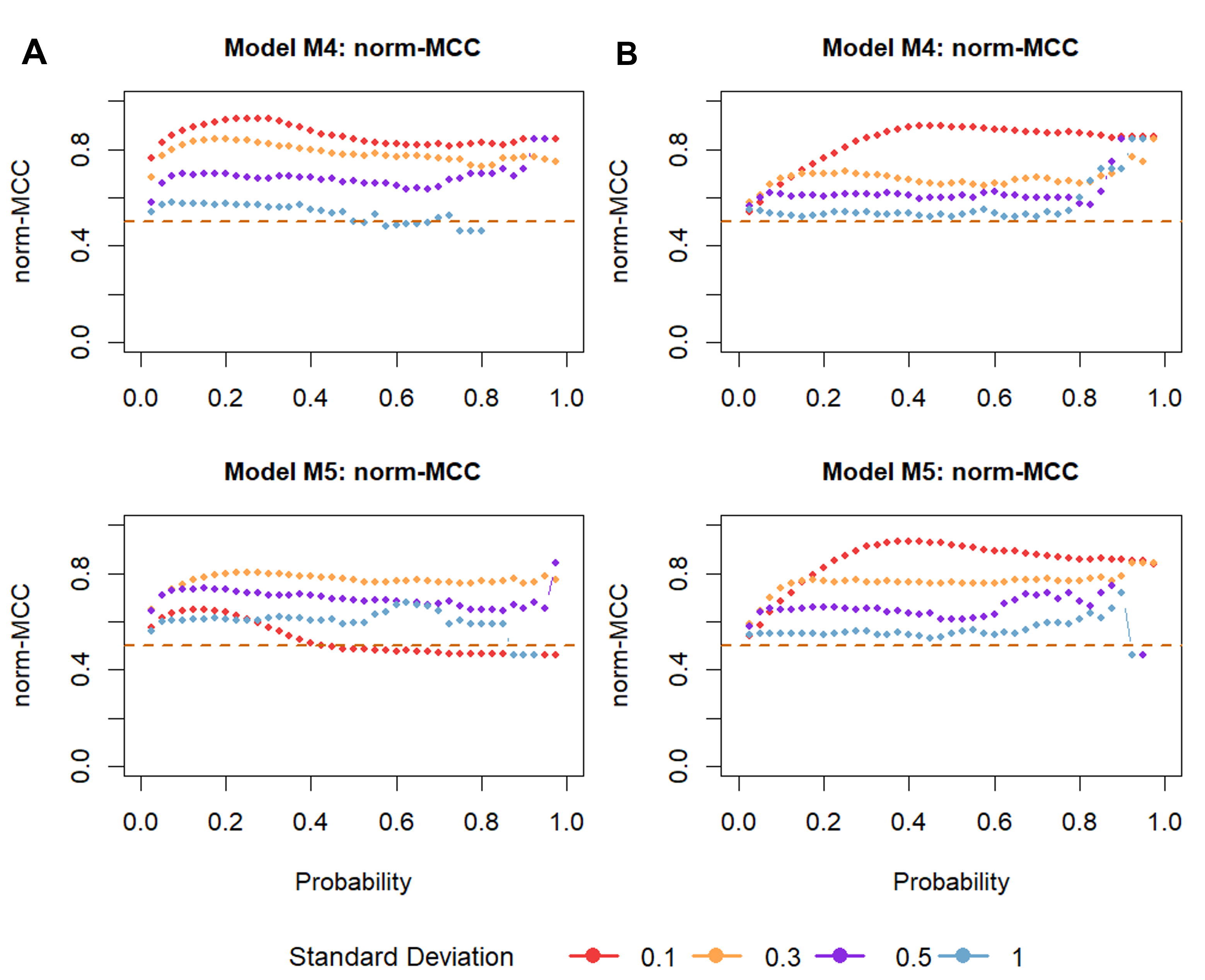
When mini growth spurts were present (models M4 and M5), the performance of changepoint analysis was assessed by calculating the area under the precision-Recall curve (PR-AUC) and norm-MCC. In contrast to the models M1, M2a, M2b, and M3, the algorithm’s performance in detecting mini growth spurts decreased with increasing measurement error (Figure 5). A considerable problem was the lack of positive predictions for higher probability thresholds. A higher measurement error seemed to enhance this effect. To calculate precision and norm-MCC values, true positive or false positive values are necessary (Table 1). When there were only negative predictions, estimation of precision and MCC values was not feasible. In order to calculate the PR-AUC, missing precision values were substituted with 0, resulting in an underestimation of the PR-AUC. Missing norm-MCC values were excluded. For small probabilities and smaller measurement error, the number of missing values was relatively small. At a probability threshold τ of 0.3 and a measurement error up to 0.3 cm, missing values were less than 20 out of 500. However, when the measurement error increased up to 1 cm, more than half of the values were missing for both models M4 and M5 (Table 2). Therefore, we consider norm-MCC to be a better indicator of the algorithm’s performance in the case of small numbers of missing values.

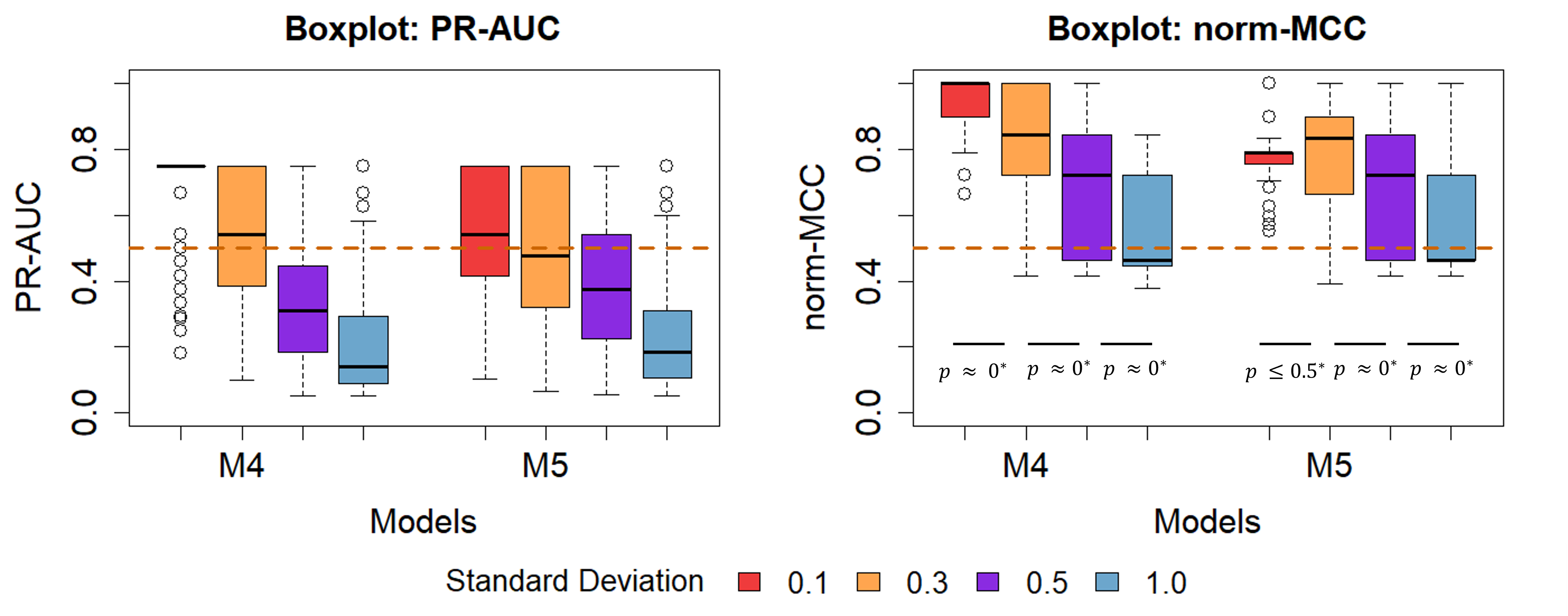
When the measurement error was small, changepoint analysis was better at detecting mini-growth spurts when linear growth was absent (M4). For a measurement error up to 0.3 cm, norm-MCC ranged between 0.8 and 0.95 for model M4 and 0.75 and 0.8 for model M5. However, ss the measurement error increased, the presence of linear growth played a subordinate role (Figure 6). Welch’s t-test suggested a significant decrease in prediction quality. As the measurement error increased, it was more difficult to detect mini growth spurts, with predictions not being better than random at measurement errors of 1 cm.

Figure 5  Assessment of changepoint analysis performance using A: Precision Recall (PR)-Curve and B: normalised Matthews correlation coefficient (norm-MCC) plotted against different probability thresholds for the models M4 and M5. SD represents measurement error. Dashed lines indicate results for a random classification.

Figure 6  Influence of the measurement error on the algorithm’s performance. SD represents measurement error. Area under the PR-Curve (left) and norm-MCC (right) are depicted for models M4 (growth spurts) and M5 (growth spurts & linear growth). Welch’s t-test was performed pairwise to assess significant difference between mean norm-MCC for different SD.

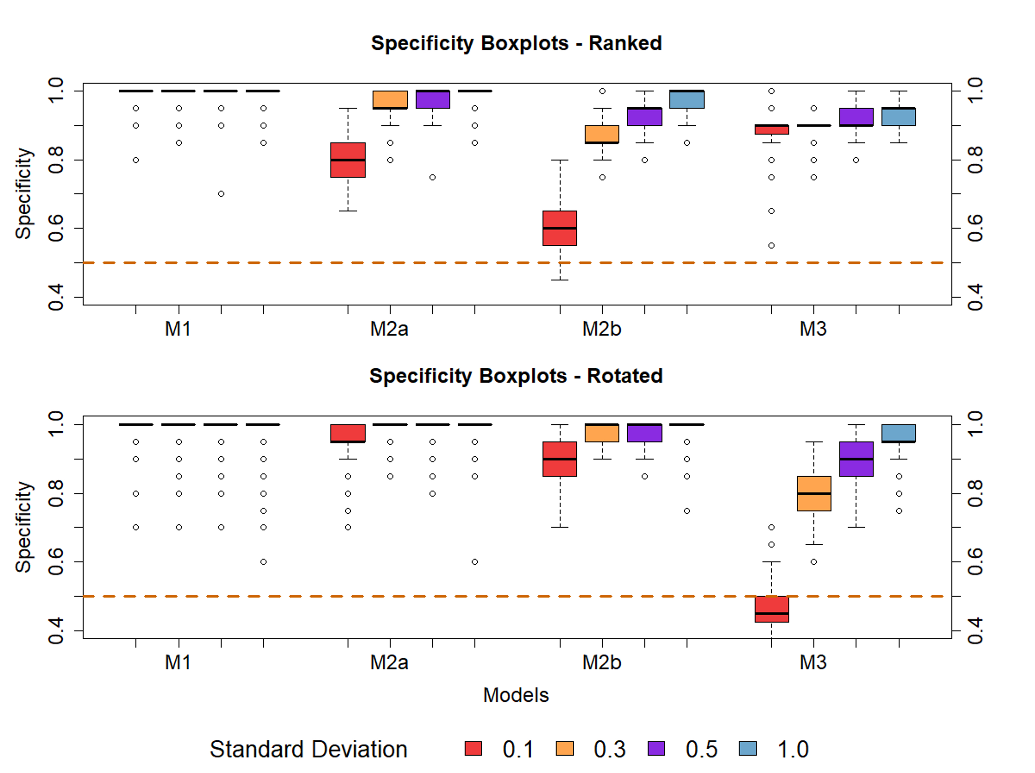
Effect of ranking and rotating on the performance of changepoint analysis

Figure 7  Specificity of changepoint analysis for A: ranked data and B: rotated data models plotted against different probability thresholds. By running 500 iterations for each model and each SD, the influence of the measurement error on the algorithm’s specificity was tested. Models depicted: M1: no growth, M2a & M2b: linear growth and M3: catch-up growth. Dashed lines indicate results for a random classification.

To compare the performance of regular changepoint analysis with changepoint analysis performed on ranked and rotated data, again specificity and norm-MCC were used for comparisons (Figure 7 and 9). Similar to regular changepoint analysis, a higher probability value as a cut-off threshold resulted in positive predictions being absent in some cases. Missing values hindered the estimation precision and norm-MCC, which require true positive or false positive predictions (Table 1). While ranking the data seemed to decrease the number of missing values for a measurement error up to 0.5 cm, rotating had quite the opposite effect (Table 2). When growth spurts and linear growth occurred together, ranking the data reduced the missing values almost by half. Rotating the time series on the other hand led to a drastic increase of missing values. Compared to regular changepoint analysis, missing values occurred at least eight times more frequently for a measurement error around 0.3 cm. If the measurement error was approximately 0.5 cm, more than half of the values were missing. The effect was greater when linear growth and growth spurts occurred at the same time.

Figure 8  Influence of the SD on the algorithm’s specificity for A: ranked and B: rotated data models. SD represents the measurement error. Models depicted: M1: no growth, M2a & M2b: linear growth and M3: catch-up growth. Dashed lines indicate results for a random classification.

Rotating the time series seemed to produce better results than ranking the time series data, except for model M3 (catch-up growth) (Figure 8). Due to the different number of missing values, the two methods cannot easily be compared. Results for ranking the data are expected to be more representative of prediction quality. This observation is reinforced by classification results of ranked data behaving similarly to regular changepoint analysis for different measurement errors (Figure 10). When the data was ranked, changepoint analysis seemed to be better at classifying catch-up growth correctly (Figure 8).

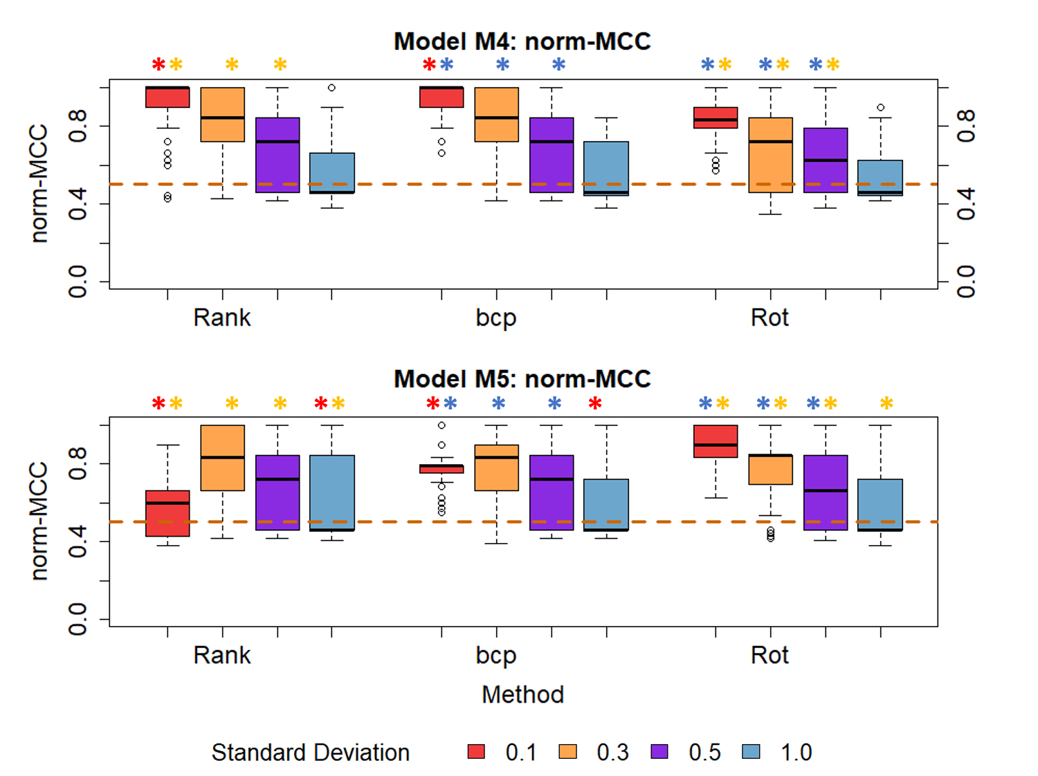
Ranking or rotating the data in advance did not seem to have a positive effect on the algorithm’s ability to detect mini growth spurts. When growth appeared only in form of growth spurts, regular changepoint analysis and ranking the data achieved the best results. Figure 10 depicts the performance of regular changepoint analysis. Differences became more obvious when the time series were rotated. In these cases, regular changepoint analysis usually offered the best results.

Figure 9  Comparison of changepoint analysis performance for ranked (A) and rotated (B) datasets. norm-MCC is plotted against different probability thresholds. Models depicted: M4 growth spurts M5 growth Spurts & linear growth. Dashed lines indicate results for a random classification.

Only when the measurement error was near 1 cm there was no difference between the different approaches. With a measurement error near 0.1 cm, rotating the time series performed best when the growth spurts appeared along linear growth. This was also the only case where ranking performed noticeably worse. When the measurement error was greater, classification was similar for all the approaches, with ranking and regular changepoint analysis performing slightly better.

Figure 10  Comparison of changepoint analysis performance between raw (bcp), ranked (Rank) and rotated (Rot) datasets. Models depicted: M4 growth spurts M5 growth spurts and linear growth. Welch’s t-test was performed pairwise to assess significant difference between mean normalised -MCC values of different methods for a given SD. Stars with the same colour indicate a significant difference between mean norm-MCC values of different methods. SD represents measurement error. Dashed lines indicate results for a random classification.

Discussion

Applicability on changepoint analysis on short-term growth

We performed Bayesian changepoint analysis on simulated growth data to test the hypothesis if changepoint analysis is able to detect mini-growth spurts and if changepoint analysis was also able to discriminate periods where growth spurts occurred from periods that lacked growth spurts. In all cases, performance of changepoint analysis highly depended on measurement error. In the absence of growth spurts, specificity of changepoint analysis increased with a higher measuring error. In 80% and 95% of the cases changepoint analysis was able to correctly identify growth without growth spurts. Though a specificity of 90% might sound good on initial read, the imbalanced nature of the dataset needs to be considered: only 10% of the datapoints were truly positives. To put this into perspective, a classifier that predicts all values as negatives would have a specificity of 0.9. Specificity values below 0.9 should therefore be viewed as undesirable (Chicco and Jurman, 2020).

At the same time however, a greater measurement error made it harder for the algorithm to detect mini growth spurts. For a measurement error up to 0.5 cm norm-MCC was between 0.7 and 0.9 and therefore much better than random classification. As the measurement error reached 1 cm, performance was no better than random. Compared to the measurement error height velocity was relatively small, reaching a maximum of 0.1 cm/day. A greater measurement error might therefore overshadow the underlying growth pattern, making it more difficult for the algorithm to detect mini growth spurts. The results show a trade-off between the algorithm’s ability to correctly detect mini growth spurts and to correctly identify growth without growth spurts.

Rotating and ranking

While preparing the data we realized that especially ranking can lead to better classification, that changepoint analysis depended more on measurement error and the model assessed at the time. Perhaps the biggest advantage of ranking was the reduction of missing values, leading to more accurate estimations. Since the number of missing values was apparently correlated with higher measurement error, limiting the effect of measurement error by ranking the time series might explain the observed positive effect. Rotating the time series seemed to increase the algorithm’s specificity. However, specificity considers only that part of negative predictions that was predicted correctly. A high specificity could be therefore the result of an overall difficulty of an algorithm to detect mini-growth spurts. We do not encourage rotating the time series, as it did have a negative effect on the classification results in most cases and increased the number of missing values. Depending on the situation we personally preferred ranking the data before using changepoint analysis.

Algorithm constraints

As a non-parametric approach, bcp does not need any distribution parameters specified. This is a particularly useful feature as mini growth spurts have only been documented in healthy neonates and small mammals (Hermanussen, 2013, 1998), but may well be present in other samples. One of the biggest issues are missing values. With increasing probability thresholds, the probability increases to correctly label a changepoint as truly positive. As it was harder for predictions to be labelled positive, positive predictions decreased up to that point where no positive predictions were left. At this point, PR-AUC and MCC could no longer be calculated. Replacing missing PR-AUC values with 0 in order to proceed with the calculation resulted in an underestimation of the PR-AUC values as shown in the boxplots. This was also true for norm-MCC values, when missing values occurred frequently. A measurement error around 0.3 cm and a probability threshold around 0.3 seemed to give an appropriate trade-off between specificity, norm-MCC and missing values. In summary, short-term growth is a complex process that still lacks adequate characterisation. The models described in this study represent simplified implementations of reality. The models give some first impressions about the applicability of changepoint analysis for short-term growth analysis. Changepoint analysis applied to real growth data is even more complex and yet needs to be tested.

Conclusion

When applied on simulated growth data, changepoint analysis was not only able to detect mini growth spurts but to also discriminate between different forms of growth including patterns that lacked growth spurts. The algorithm’s performance highly depends on measurement error and growth pattern. Ranking or rotating the data beforehand did not significantly improve the algorithm’s performance. We believe that changepoint analysis is a promising and new tool for the analysis of short-term growth and are eager to asses it’s performance on real growth data.

References

Aminikhanghahi, S./Cook, D. J. (2017). A survey of methods for time series change point detection. Knowledge and Information Systems 51, 339–367. https://doi.org/10.1007/s10115-016-0987-z.

Bär, C. (2018). Lineare Algebra und analytische Geometrie. Wiesbaden, Springer Fachmedien Wiesbaden. https://doi.org/10.1007/978-3-658-22620-6.

Barry, D./Hartigan, J. A. (1993). A Bayesian Analysis for Change Point Problems. Journal of the American Statistical Association 88, 309–319. https://doi.org/10.1080/01621459.1993.10594323.

Bubitzky, W./Granzow, M./Berrar, D. P. (Eds.) (2007). Fundamentals of data mining in genomics and proteomics. New York, Springer.

Caino, S./Kelmansky, D./Lejarraga, H./Adamo, P. (2004). Short-term growth in healthy infants, schoolchildren and adolescent girls. Annals of Human Biology 31, 182–195. https://doi.org/10.1080/03014460310001652220.

Chicco, D. (2017). Ten quick tips for machine learning in computational biology. BioData Mining 10, 35. https://doi.org/10.1186/s13040-017-0155-3.

Chicco, D./Jurman, G. (2020). The advantages of the Matthews correlation coefficient (MCC) over F1 score and accuracy in binary classification evaluation. BMC Genomics 21, 6. https://doi.org/10.1186/s12864-019-6413-7.

Erdman, C./Emerson, J. W. (2007). bcp: An R Package for performing a Bayesian analysis of change point problems. Journal of Statistical Software 23. https://doi.org/10.18637/jss.v023.i03.

Hermanussen, M. (Ed.) (2013). Auxology. Stuttgart, Schweizerbart Science Publishers.

Hermanussen, M. (1998). The Analysis of short-term growth. Hormone Research in Paediatrics 49, 53–64. https://doi.org/10.1159/000023127.

Hoffman, M. M./Chang, C./Chicco, D. (2020). The MCC-F1 curve: a performance evaluation technique for binary classification. arXiv. https://doi.org/10.48550/arXiv.2006.11278.

Lalkhen, A. G./McCluskey, A. (2008). Clinical tests: sensitivity and specificity. Continuing Education in Anaesthesia Critical Care & Pain 8, 221–223. https://doi.org/10.1093/bjaceaccp/mkn041.

Lin, J./Khade, R./Li, Y. (2012). Rotation-invariant similarity in time series using bag-of-patterns representation. Journal of Intelligent Information Systems 39, 287–315. https://doi.org/10.1007/s10844-012-0196-5.

Matthews, B. W. (1975). Coparison of the predicted and observed secondary structure of T4 phage lysozyme. Biochimica et Biophysica Acta - Protein Structure 405 (2), 442-451 https://doi.org/10.1016/0005-2795(75)90109-9.

Novine, M./Mattsson, C. C./Groth, D. (2022). Network reconstruction based on synthetic data generated by a Monte Carlo approach. Human Biology and Public Health 3. https://doi.org/10.52905/hbph2021.3.26.

Olshen, A. B./Venkatraman, E. S./Lucito, R./Wigler, M. (2004). Circular binary segmentation for the analysis of array-based DNA copy number data. Biostatistics 5, 557–572. https://doi.org/10.1093/biostatistics/kxh008.

Rösler, A./Scheffler, C./Hermanussen, M./Gasparatos, N. (2022). Practicability and user friendliness of height measurements by proof of concept APP using Augmented Reality, in 22 healthy children. Human Biology and Public Health 2. https://doi.org/10.52905/hbph2022.2.48.

Schrade, L./Scheffler, C. (2013). Assessing the applicability of the digital laser rangefinder GLM Professional® Bosch 250 VF for anthropometric field studies. Anthropologischer Anzeiger 70, 137–145. https://doi.org/10.1127/0003-5548/2013/0223.

Schroth, C./Siebert, J./Groß, J. (2021). Time traveling with data science: focusing on change point detection in time series analysis (Part 2). Available online at https://www.iese.fraunhofer.de/blog/change-point-detection/ (accessed 11/21/2022).

Siebert, J./Groß, J./Schroth, C. (2021). A systematic review of Python packages for time series analysis. Engineering proceedings 5. https://doi.org/10.3390/engproc2021005022.