Network reconstruction based on synthetic data generated by a Monte Carlo
approach
Masiar Novine ✉
✉
University of Potsdam, Institute of Biochemistry and Biology, Bioinformatics
Group, 14469 Potsdam, Germany.
Cecilie Cordua Mattsson
ADBOU, Institute of Forensic Medicine, University of Southern Denmark,
Campusvej 55, DK 5230 Odense M, Denmark.
Detlef Groth
University of Potsdam, Institute of Biochemistry and Biology, Bioinformatics
Group, 14469 Potsdam, Germany.
DOI: https://doi.org/10.52905/hbph2021.3.26
Abstract
BackgroundNetwork models are useful tools for researchers to simplify and understand investigated
systems. Yet, the assessment of methods for network construction is often uncertain.
Random resampling simulations can aid to assess methods, provided synthetic data exists
for reliable network construction.
ObjectivesWe implemented a new Monte Carlo algorithm to create simulated data for network
reconstruction, tested the influence of adjusted parameters and used simulations to
select a method for network model estimation based on real-world data. We hypothesized,
that reconstructs based on Monte Carlo data are scored at least as good compared to a
benchmark.
MethodsSimulated data was generated in R using the Monte Carlo algorithm of the
mcgraph package. Benchmark data was created by the
huge package. Networks were reconstructed using six estimator
functions and scored by four classification metrics. For compatibility tests of mean
score differences, Welch’s t-test was used. Network model estimation
based on real-world data was done by stepwise selection.
SamplesSimulated data was generated based on 640 input graphs of various types and sizes. The
real-world dataset consisted of 67 medieval skeletons of females and males from the
region of Refshale (Lolland) and Nordby (Jutland) in Denmark.
ResultsResults after t-tests and determining confidence intervals (CI95%) show,
that evaluation scores for network reconstructs based on the mcgraph package were at least
as good compared to the benchmark huge. The results even indicate slightly better scores on
average for the mcgraph package.
ConclusionThe results confirmed our objective and suggested that Monte Carlo data can keep up
with the benchmark in the applied test framework. The algorithm offers the feature to
use (weighted) un- and directed graphs and might be useful for
assessing methods for network construction.
Keywords: Monte Carlo method, network science, network reconstruction, mcgraph, random sampling, linear enamel hypoplasia
Conflict of Interest: There are no
conflicts of interest.
Citation: Novine, M. / Mattsson, C. / Groth, D. (2021). Network reconstruction based on synthetic data generated by a Monte Carlo
approach. Human Biology and Public Health 3. https://doi.org/10.52905/hbph2021.3.26.
Copyright: This is an open access article distributed under the terms of the Creative Commons Attribution License which permits unrestricted use, distribution, and reproduction in any medium, provided the original author and source are credited.
Received: 02-11-2021 | Accepted: 31-03-2022 | Published: 16-06-2022
Take home message for students
Random sampling is a simple, but effective approach. It can be used in the context of
network analysis to access the quality of network reconstruction methods.
Contents
Introduction
Networks are visualized by graphs, where variables are represented as nodes, while
associations are depicted as edges (i.e., lines between nodes). Using such a form of
representation, graphs can help to simplify a complex system by focusing on the
relationships of its members (Barabási and Pósfai
2016) (e.g., see figure 1 for an example,
illustrating some advantages of graph models in comparison to alternative ways of
visualization). Network analysis uses graph theory to investigate the structure of networks.
In the context of social science, social network analysis is used to analyze interactions of
social members, called actors (nodes) and focuses on their relationships (edges).
Associations can represent communication, exchange of goods or emotional affection in the
case of friendship networks (Wasserman and Faust
1994). Next to the static understanding of networks, temporal networks transmit
changes of network structures over time. Snapshots of networks at consecutive time points
can be analyzed by concepts of temporal correlation or temporal overlap (Nicosia et al. 2013). The first denotes with which
probability associations remain over time, while the second addresses the time-dependent
similarity of networks. Such approaches can be useful to uncover dynamic systems like
modeling trade movements of livestock (Büttner et al.
2016).
In the context of public health, network medicine investigates the interrelationship of
hierarchies of multiple networks (i.e., social, disease and metabolic / genetic networks) to
uncover phenomena like disease (Barabási et al.
2011; Loscalzo et al. 2017). For example,
while there is a genetic influence on obesity (Frayling
et al. 2007), the influence of social factors like friendship on the risk of a
person becoming obese could be shown to be more important by considering social and
underlying genetic networks. Obesity clusters in social communities made of friendship and
family networks (Christakis and Fowler 2007; Barabási 2007).
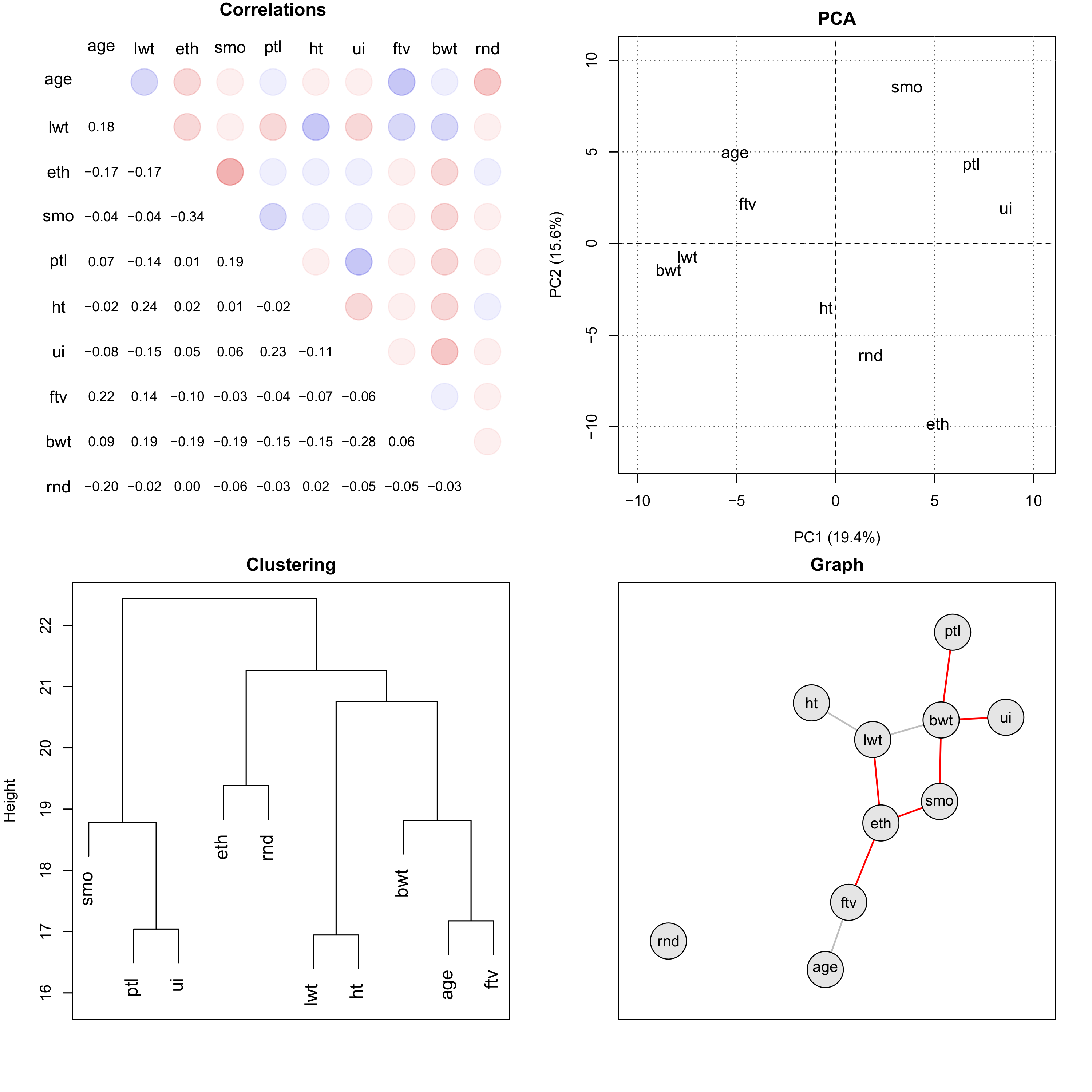
Figure 1 Comparison of multivariate data techniques. Next to the correlations, the results
of a PCA, a dendrogram based on clustering and a graph are depicted using the same
example data set. The set contains data of variables related to the health status of 189
children and their mothers, collected at Baystate Medical Center, Springfield, Mass
during 1986: age - mother’s age in years, lwt - mother’s weight in pounds at last
menstrual period, eth - mother’s ethnicity (1 = white, 2 = black, 3 = other), smo -
smoking status during pregnancy (0 = no, 1 = yes), ptl - number of previous premature
labours, ht - history of hypertension (0 = no, 1 = yes), ui - presence of uterine
irritability (0 = no, 1 = yes), ftv -number of physician visits during the first
trimester, bwt birth weight of child in grams, rnd - some random uncorrelated data. For
graph construction the St. Nicolas House algorithm was used (Groth et al. 2019; Hermanussen
et al. 2021).
Network construction methods
Constructing network models usually requires information about the relevance of
particular associations between certain variables. Selecting the relevant variables thus,
is crucial. Stepwise regression (Heinze et al.
2018) based on each node can be used but this approach requires selecting
thresholds and by including / removing one variable at a time seriously biases basic
statistics of regression analysis, leading to upward biased values, too low standard errors for regression
coefficients, too low -values and too large absolute values for coefficients
(Copas and Long 1991; Harrell 2001). Some of the problems can be solved by using graphical
lasso for regulating coefficients (Friedman et al. 2008) and stability selection (Meinshausen and Bühlmann 2006; Meinshausen and
Bühlmann 2010). Other approaches calculate the correlation matrix based on all
variables and apply (hard) correlation thresholds to filter relevant associations (Rice et al. 2005; Batushansky et al. 2016; Sulaimanov and Koeppl
2016) or use power transforms to perform soft thresholding (Zhang and Horvath 2005; Ghazalpour
et al. 2006; Langfelder and Horvath
2008). The later approach aims to avoid loss of information by binarization.
St. Nicolas House Analysis (SNHA) constructs networks based on
association chains of variables based on their correlations. The method
has advantages as it is non-parametric and there is no need to specify a selection
threshold for including variables (Groth et al.
2019; Hermanussen et al. 2021).
Using simulated data for assessment of network construction methods
Evaluating the applied method is critical when constructing network models. Estimating
the scale of the possible error becomes difficult, because the interactions of variables
in a network might be complex. Motivated by the fact, that randomized resampling
approaches like bootstrapping are routinely applied for statistical analysis to
empirically determine error terms or confidence intervals (Efron and Tibshirani 1986), we think, that a simulation-driven
approach could aid assessing a certain network construction method. We use an approach
based on the Monte Carlo method (Metropolis and Ulam
1949) due to its simplicity. We describe the approach in the method section in
more detail.
Our approach allows for flexible random data generation on pre-defined graph structures,
which is superior to most example data provided by statistical software (e.g., R). We want
to provide a simple tool to uncover strengths and limitations of methods. In view of the
notion, that “the art of data analysis is about choosing and using
multiple tools” (Harrell 2001), our approach is
embedded in a broader framework of statistical analyses.
Our presented analysis proceeded as follows: We generated synthetic data based on
pre-defined network structures of various network types and sizes, performed network
reconstruction and finally evaluated the network reconstructs by binary classification.
Such a testing framework can identify suitable candidate models or identify weaknesses of
modeling approaches by investigating on how precise and sensitive predictions of
associations between the variables are.
We tested the hypothesis, that network reconstructs based on the Monte Carlo approach are
scored at least as good compared to a benchmark. For comparison, we used the data
generation function of the R package huge. We also altered parameters of
the Monte Carlo function to assess their influence on scores of network reconstructs.
Finally, we applied a well-scored network construction method to construct a network model
based on real-world data (Mattsson 2021).
Samples and methods
Software
For most of the computations and programming we used the programming language R (R Core Team 2021) version 4.0.4. Time critical parts
were implemented in C++ via the interfaces Rcpp (Eddelbuettel and François 2011) version 1.0.7 and
RcppArmadillo (Eddelbuettel and
Sanderson 2014) version 0.10.7.0.0, enabling access to the C++ library Armadillo
(Sanderson and Curtin 2016), (Sanderson and Curtin 2018) version 10.6. Embedding
data into the manuscript and formatting of tables was done by dynamic report generation
using knitr (Xie 2021) version
1.36 and xtable (Dahl et al.
2000) version 1.8-4. We used our R package mcgraph (Groth and Novine 2022) version 0.5.0 for most of the
computational work, including synthetic data generation, data imputation, creation of
network structures, estimation of networks, evaluation of estimates and graph
visualization. As a benchmark for the Monte Carlo data, the huge package
(Zhao et al. 2012) version 1.3.5 was used.
Statistical analysis and graphics were done using R standard packages and
ggplot2 (Wickham 2016) version
3.3.5.
Classification metrics for assessment of network reconstructs
Table 1 Summary of metrics used for the evaluation of classification results. The formula
for the calculation of the Area Under the ROC curve and PRC is based on the trapezoid
rule. The variable denotes the number of classification results, including
those points located at (0, 0) and (1, 1) in the ROC curve plot, which are set as
start and end values. For the Precision-Recall Curve (PRC) those coordinates are
switched. For MCC a normalized version based on (Cao
et al. 2020) is given, scaling it to the range of 0 to 1. Next to the formula
for the calculation, the best and the worst possible scores for each metric are
included.
| Metric |
Abbreviation |
Calculation |
Worst |
Best |
| Sensitivity |
TPR |
|
0 |
1 |
| Specificity |
TNR |
|
0 |
1 |
| Precision |
PPV |
|
0 |
1 |
| False-Positive Rate |
FPR |
|
1 |
0 |
| Area Under the ROC curve |
AUC |
|
0 |
1 |
| Area Under the PRC |
PR-AUC |
|
0 |
1 |
| Balanced Classification Rate |
BCR |
|
0 |
1 |
| Matthews Correlation Coefficient |
MCC |
|
-1 |
1 |
| Normalized Matthews Correlation Coefficient |
norm-MCC |
|
0 |
1 |
We reframed the task of network reconstruction as a binary classification problem. Based
on raw data, an estimator function (i.e., a classifier) was applied to classify edges as
being present (positive case) or absent (negative case). By comparing the classification
results to the true network structure, the classification can be evaluated.
We briefly defined the possible outcomes of the classification:
| • | true-positive (TP): correct classification of an edge as being present |
| • | true-negative (TN): correct classification of an edge as being absent |
| • | false-positive (FP): incorrect classification of an edge as being present |
| • | false-negative (FN): incorrect classification of an edge as being absent |
For evaluation we used four metrics (see Table 1
for a detailed list):
| 1. | AUC, Area Under the Receiver Operating Characteristic (ROC) curve (Hanley and McNeil 1982), sensitivity (TPR)
plotted against FPR. |
| 2. | PR-AUC, area under the Precision-Recall Curve (PRC), precision (PPV) plotted against
sensitivity (TPR). |
| 3. | averaged Balanced Classification Rate (BCR) |
| 4. | averaged and normalized variant of Matthews Correlation Coefficient (norm-MCC) (Matthews 1975) |
Each classification metric is based on another scoring scheme, so that classification
results should eventually be different. In general, for metrics in the range of 0 to 1,
values of 0.5 indicate classification results not better than random. In ROC and PRC
plots, this is indicated by the baseline diagonal. Mostly, networks are sparse, so that
the set of underlying classes is imbalanced (i.e., the number of absent edges is much
higher than that of present ones). In such cases PR-AUC is preferred over AUC, because PRC
plots capture the relationship between PPV and TPR, both concerned with the fraction of TP
among prediction outcomes. AUC on the other hand relies on FPR, which has the number of TN
cases in the denominator. This number will be overwhelmingly higher in the case of sparse
networks and will push the value of FPR towards 0 (i.e., best score) leading to an overly
optimistic and misleading AUC (Cao et al. 2020;
Chicco and Jurman 2020). Next to AUC and
PR-AUC, we additionally used BCR and norm-MCC to (1) express the underlying
characteristics of the data better (2) illustrate and control for differences of the
scoring values and (3) compare trends across metrics.
Proposed Monte Carlo method for simulated data generation
Input graphs
The input for the data generation algorithm is either an (weighted) un- or directed
graph. Assume an initial graph with a set of nodes with and a set of edges with . Computationally, we represent the graph in form of an
adjacency matrix (i.e., a binary square matrix with the dimensions
, with being the number of nodes given by the size of the set
. We denote , such that is a directed edge between node and . Consequently, an undirected edge is given as
. We define a weight function , such that is a weighted edge. We call an edge between
and simple, if . Throughout our analysis, we only considered simple
edges. Edges are indicated by non-zero entries in the according field of the matrix.
Positive or negative edges indicate positive or negative associations between the
according variables, respectively. A directed graph is represented by a non-symmetric
adjacency matrix, while the adjacency matrix of an undirected graph is symmetric (i.e.,
dividing the matrix along the diagonal leads to the two halves behaving as image and
reflection). Finally, we defined the relationship of two connected nodes as follows: A
source node is a node, where the edge originates from, and the target node is a node
where the according edge ends in. Sometimes we call the source incoming
neighbor and the target outgoing
neighbor.
Steps of Monte Carlo sampling
Listing 1 Pseudocode for the Monte Carlo data generation algorithm
Input: adjacency matrix
Output: matrix
procedure monteCarlo(, , , , )
Create empty , where:
number of nodes
number of samples per node
for to do
Vector with data randomly drawn from
for to do
foreach in shuffle() do
foreach in shuffle(neighbors()) do
Proportion source value for updated target value
weightedMean(, , , )
if () then
else
endfor
endfor
Add to values
endfor
Assign values of to the -th column of
endfor
return
Monte Carlo sampling is done based on the following iterative approach:
| 1. | data values are randomly chosen from a normal
distribution with a given mean and a given standard deviation
based on the probability density function |
| 2. |
|
| 3. | and assigned to each node in the set . |
| 4. | A source node is randomly chosen from the set without replacement and all its outgoing neighbors
are found. |
| 5. | From the set of outgoing neighbors, a target node is randomly chosen and the
weighted mean between source and target is calculated based on |
| 6. |
|
| 7. | The initial value of the target is then replaced by the newly calculated value. By
adjusting a proportion argument (prop) the user can determine, how
the mean is weighted (e.g., setting prop = 0.1 would indicate, that
the updated value for the target node is calculated by taking 90% of its prior value
and 10% of the value of the source node and then multiplying the proportion with the
absolute values of the respective edge weights). Hence, over time the value for the
target becomes more correlated to the value of the source. |
| 8. | For a given number of iterations, steps 2 and 3 are repeated for all the nodes in
and the total number of outgoing neighbors of each
chosen source node, respectively. All the steps are repeated
times, where corresponds to the number of data values for each
node. In the end, the result of the procedure is an data matrix. In listing 1 the pseudocode of the approach is given. |
| 9. | When calculating the weighted mean, the absolute edge weight is also considered,
which will influence the mean calculation. If edge weights are negative, first the
weighted mean is calculated as previously, but subtracted from twice the value of
the target node to get its updated value, making them anti-correlated. It is
important to note, that the algorithm defines a source-to-target relationship for
each pair of connected nodes, independent of the input graph being directed or
not. |
Monte Carlo algorithm – How synthetic data is created
The implementation of the algorithm offers several arguments for which input values can
be varied to change the shape of the synthetic data (see Table 2 Appendix).
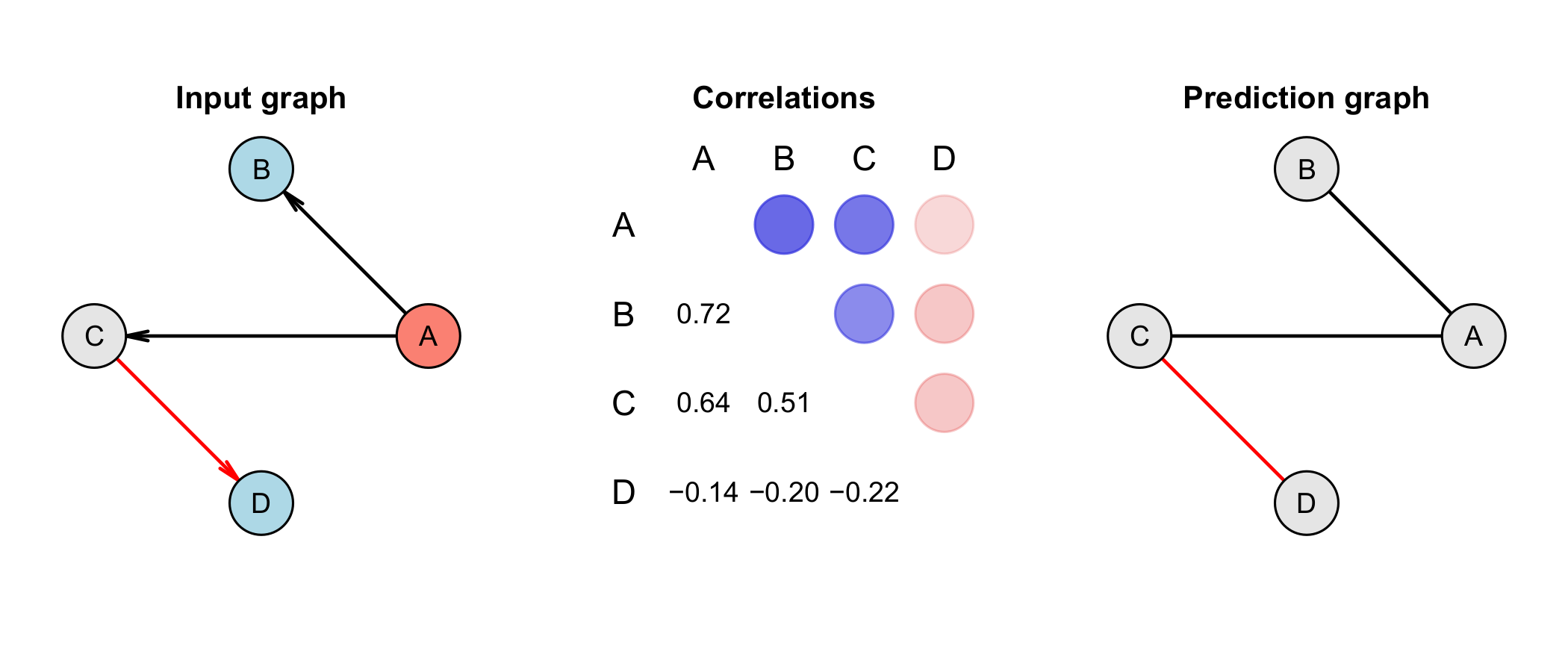
Figure 2 Graphs and data generation. An input graph with its resulting correlation
matrix of synthetic data generated for a small network. The input graph with 4 nodes
and 3 directed edges (left), the correlation matrix (center) based on synthetic data
generated for this small network and a predicted undirected graph based on the
underlying data (right). A is a confounder and has a strong positive correlation to
B and C. Due to the negative correlation between C and D, both, A and B are also
negatively correlated to D, illustrating the influence of indirect associations on
the pair-wise correlation of two nodes. The data was generated by the here presented
algorithm using the Monte Carlo method. Red edges indicate negative correlations. In
the correlation matrix, positive correlations are indicated with a blue circle,
while negative correlations are shown as a red circle. The strength of the
correlation is depicted by the strength of the color.
We used the example in figure 2 to illustrate
the mechanics of data creation. We assumed simple edges and a value for the influence of
the source node on the target (, 10%). For details of the algorithm see Listing 1. The algorithm creates a vector with
random values from for each variable. In the depicted directed graph,
(source) influences (target) positively indicated by a directed edge from
to . For simplicity, let us only consider the first element
of the vectors of and given for example as and . Based on the updating rule the new value
is the weighted mean between the two values, so that
. Consequently, after multiple iterations the vectors of
and become similar and are positively correlated. The
algorithm adds noise after each iteration to avoid that correlations develop too
quickly.
Take the case, where only influences negatively without any other influence present (i.e., for
the moment we neglect that influences positively). Assume and . In the first step, we calculated the weighted mean
between the two values, so that . In the second step we subtracted this result from twice
the value of to get to its updated value, so that
. Hence, and become more anti-correlated over time.
Note, that the example network in figure 2 is more complex: is a confounding variable. It positively influences both
and . In consequence, and become correlated due to their shared association with
. Additionally, this confounding effect leads to an
anti-correlation between , and due to the shared association with
(see the correlation matrix in figure 2).
Methods used for network reconstruction
We used following functions for network (re)construction from the
mcgraph package:
mcg.ct: Simple (hard) correlation thresholding with hard based on a
threshold to prune the correlated data values and to encode the
correlation matrix into a binary adjacency matrix.
mcg.lvs: Stepwise regression (i.e., forward variable selection). One
variable after the other was used as a response variable and we preselected the
k highest correlated variables of each response as candidates using
Pearson correlation. The selection was based on minimizing AIC and at the same time
maximizing , while the change in has to be equal or larger than a given threshold.
mcg.rpart: Forward variable selection using regression trees (Breiman et al. 1984). We again only used the
k highest correlated variables for each response variable using
Spearman correlation.
Additionally, we used following implementations of the huge package:
huge.ct: correlation thresholding
huge.glasso: graphical lasso (Friedman et al. 2008)
huge.mb: stability selection (Meinshausen and Bühlmann 2006)
Analysis of parameters of the Monte Carlo algorithm
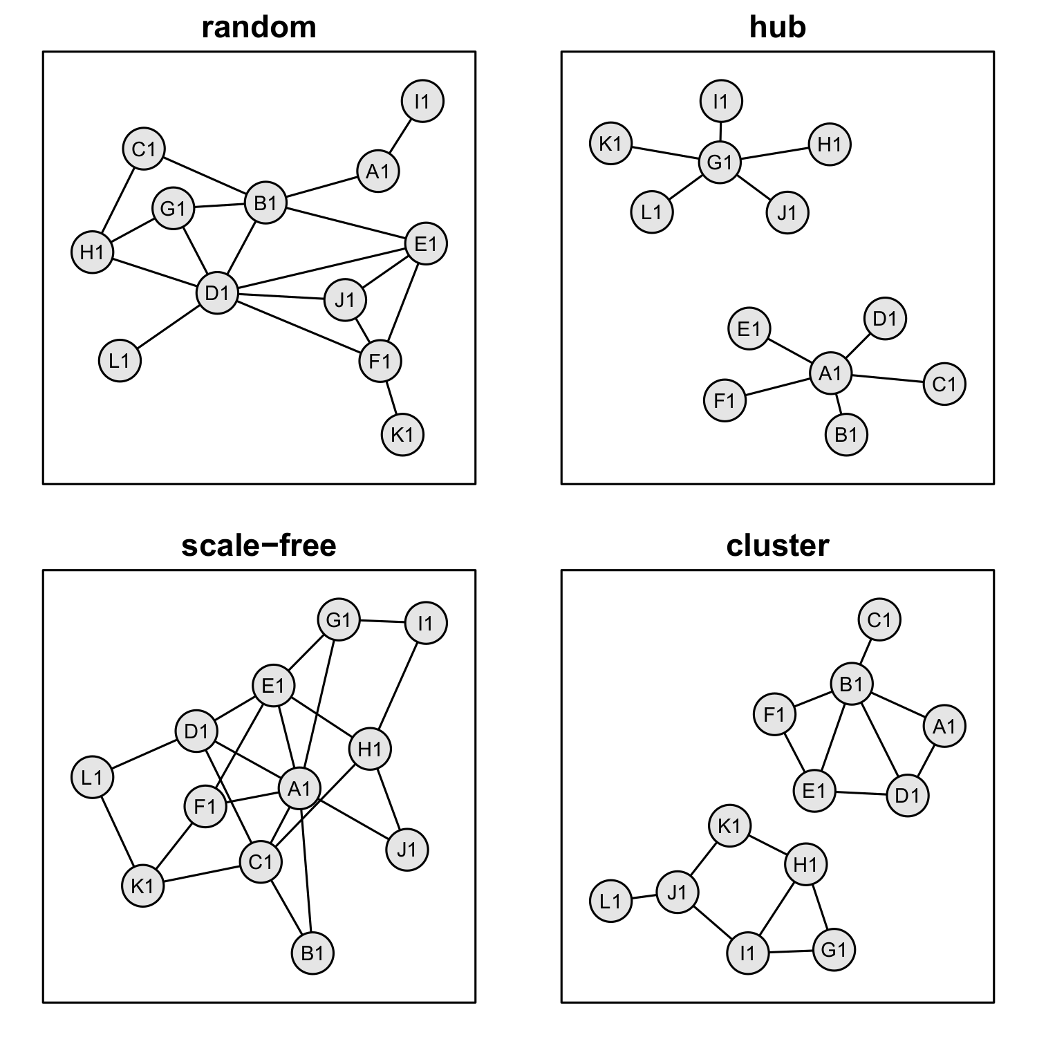
Figure 3 Examples of general network types. In our simulation analysis, we used the four
network types random, hub, scale-free and cluster to test the influence of the network
structure on the quality of reconstructs.
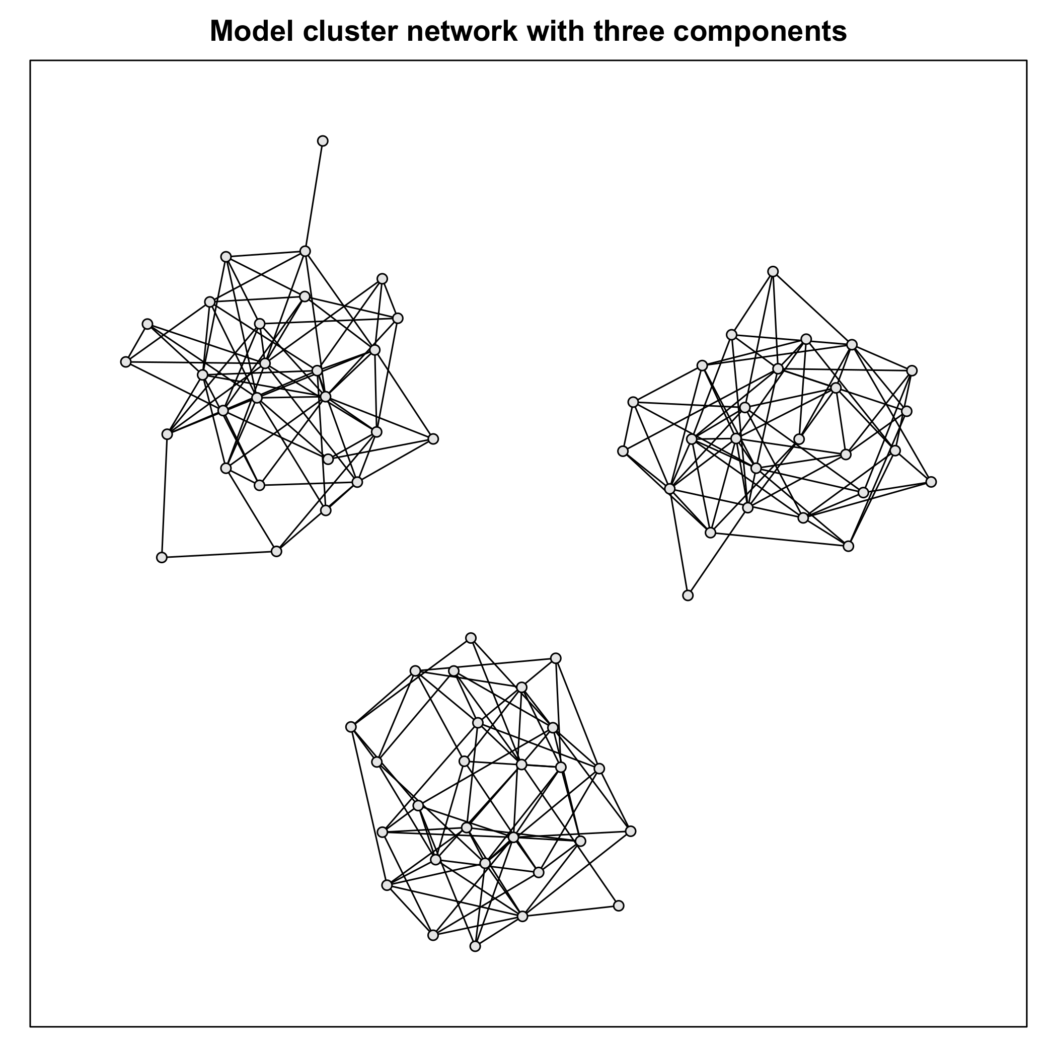
Figure 4 Model cluster network. The depicted cluster network with three components was
used as a model network for determining the influence of four key parameters of the
Monte Carlo data generation algorithm: iter, prop, noise and the number of samples per
variable n.
Based on a cluster network (80 nodes, 235 edges, 3 components) shown in figure 4 we
tested the n, iter, prop and
noise (see Table 2 Appendix)
arguments to investigate their influence on PR-AUC scores of network reconstructs. In our
simulation test, PR-AUC scores for reconstructs of the cluster network were among the
worst, even by methods for which scores has been higher on average. Hence, the network was
selected as a suitable candidate for optimization tests. For network reconstruction we
used forward variable selection and evaluate the reconstructs. We chose settings for the
parameters based on a reasonable range and plot PRCs to illustrate the influence on the
reconstructs.
Comparative analysis of Monte Carlo
data using network reconstruction
Based on the network types random, scale-free, hub, and cluster (exemplified in figure 3)
network reconstruction was done. We used undirected graphs with simple edges. In a first
step, the given networks were generated by the huge.generator function
using the specified graph sizes (20, 40, 80, 400) shown in figure 5. We used the default
values for parameters of the function with the number of samples per variable set to
. The number of edges was internally determined by the
function, as well as the number of components for cluster and hub networks. The generated
adjacency matrix was parsed to the mcgraph Monte Carlo function
mcg.graph2data to use the same input graph. The parameters of the
function were set to , , and . The classification thresholds, which denote
cutoffs of the mcgraph estimators were
kept in a reasonable range, spanning from 0 to about 0.1. The values for the tuning
parameter of the huge estimators were automatically
calculated as advised by the reference manual (Jiang
et al. 2021). Network reconstruction was performed based on the implementations
described in the previous section (see Methods used for
network reconstruction). We evaluated the reconstructs by AUC, PR-AUC,
BCR and norm-MCC. To determine significance in mean differences, Welch’s
-test was performed as described in literature (Berrar et al. 2007; Wasserman 2013).
A real-world example – Analysis of the relationship of linear enamel hypoplasia and
bone growth
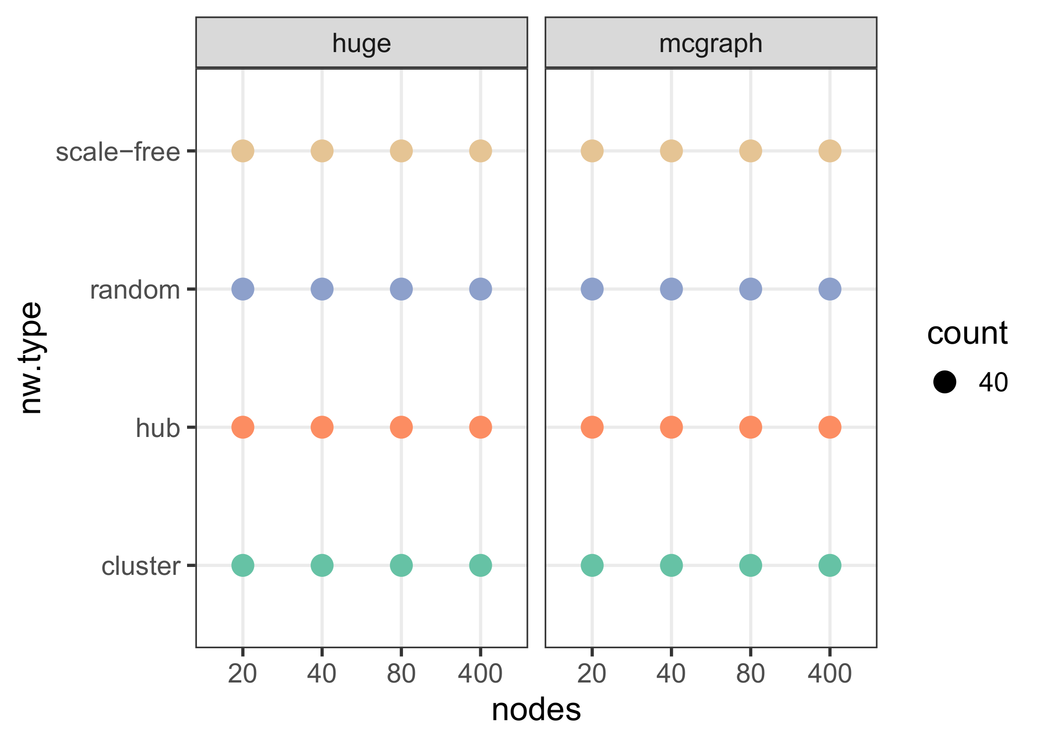
Figure 5 Number of samples for each network type. Regarding both packages, we used random,
cluster, hub and scale-free (Barabàsi-Albert) graphs, with number of nodes 20, 40, 80,
400. For each generated graph structure 40 individual graphs were randomly generated,
such that the total number of input graphs was 640. After data generation by the huge
function (huge.generator), the adjacency matrix of each graph was given to the Monte
Carlo data generation function of mcgraph (mcg.graph2data). Subsequently, network
reconstruction was performed, followed by evaluation of the
reconstructs.
Sample
We used data from (Mattsson 2021) collected in
late 2020 (ADBOU, Unit of Anthropology, Department of Forensic Medicine,
University of Southern Denmark). The data set consisted of observations of 67 medieval
skeletons of Danish females and males from the region of Refshale (Lolland) and Nordby
(Jutland) in Denmark. It included the age of death, which was estimated based on
different age markers using a standard method (Milner
and Boldsen 2012; Tarp 2017) and the
sex of the individuals. Additionally, it contained measurements of the length of the
pairs of humeri, radial bones, thigh bones (femora) and shank bones (tibiae). Presence
of LEH in the canines of both sides of the upper and lower denture was included as a
binary assessment.
Sample preparation
Prior to further analysis, we performed data imputation based on regression trees. We
calculated the ratio between the lengths of the pairs of humeri and radial bones and the
ratio between the lengths of the pairs of thigh bones and shank bones for each sample.
Furthermore, we determined the average of the lengths of each bone type.
Network estimation
Our version of stepwise regression was selected based on relatively high scores in our
simulation analysis described in the prior section. Using LEH scores of canines of the
upper and lower denture, ratios of long bones of arms and legs, lengths of humeri,
tibiae, femora, radial and sex, we estimated a network to investigate the relationship
between the presence of LEH and the growth of the selected bones. The threshold
, which is used for model selection by the stepwise
regression algorithm was kept at the default value of 0.04. denoted the difference of the values of a model excluding and a model including a
candidate variable (i.e., it is the value by which the regression model must improve to
justify the inclusion of a variable). We set the number of most correlated candidates
per response variable to the default value of . The other selection criterion was a smaller value for
Akaikes Information Criterion (AIC) (Akaike
1974; Sakamoto et al. 1986).
Results

Figure 6 Testing the influence of key parameters of the Monte Carlo data generation
function. We performed network reconstruction using stepwise regression based on the
cluster network depicted in figure 4. Reconstructs were evaluated by PR-AUC. Four
set-ups were tested and in each the number of iterations was doubled (i.e., we used 15,
30, 60 and 120 number of iterations). In (A) we varied the prop argument using the
values 5%, 10% and 20%. In (B) the random noise added was 0.1, 1 and 10, respectively.
In (C) we varied the values for the number of samples for each variable (100, 200,
1000). The diagonal line is the baseline indicating the result for a random
classification.
The influence of parameters of the Monte Carlo function on the shape of the simulated data
was assessed by comparing PR curves of network reconstructs (Figure 6).
A higher number of iterations and a lower value of prop improved PR-AUC
scores.
The effect of noise on the scores was especially dependent on the number of iterations:
While for lower number of iterations (15, 30) the noise level had an impact on scores, such
that less noise let to higher scores, this effect disappeared by increasing the number of
iterations (60, 120). Higher numbers of samples per variable had the most positive effect on
scores: While by using 100 samples per variable, scores were equal to a random
classification, the scores improved substantially by using 1000 samples.
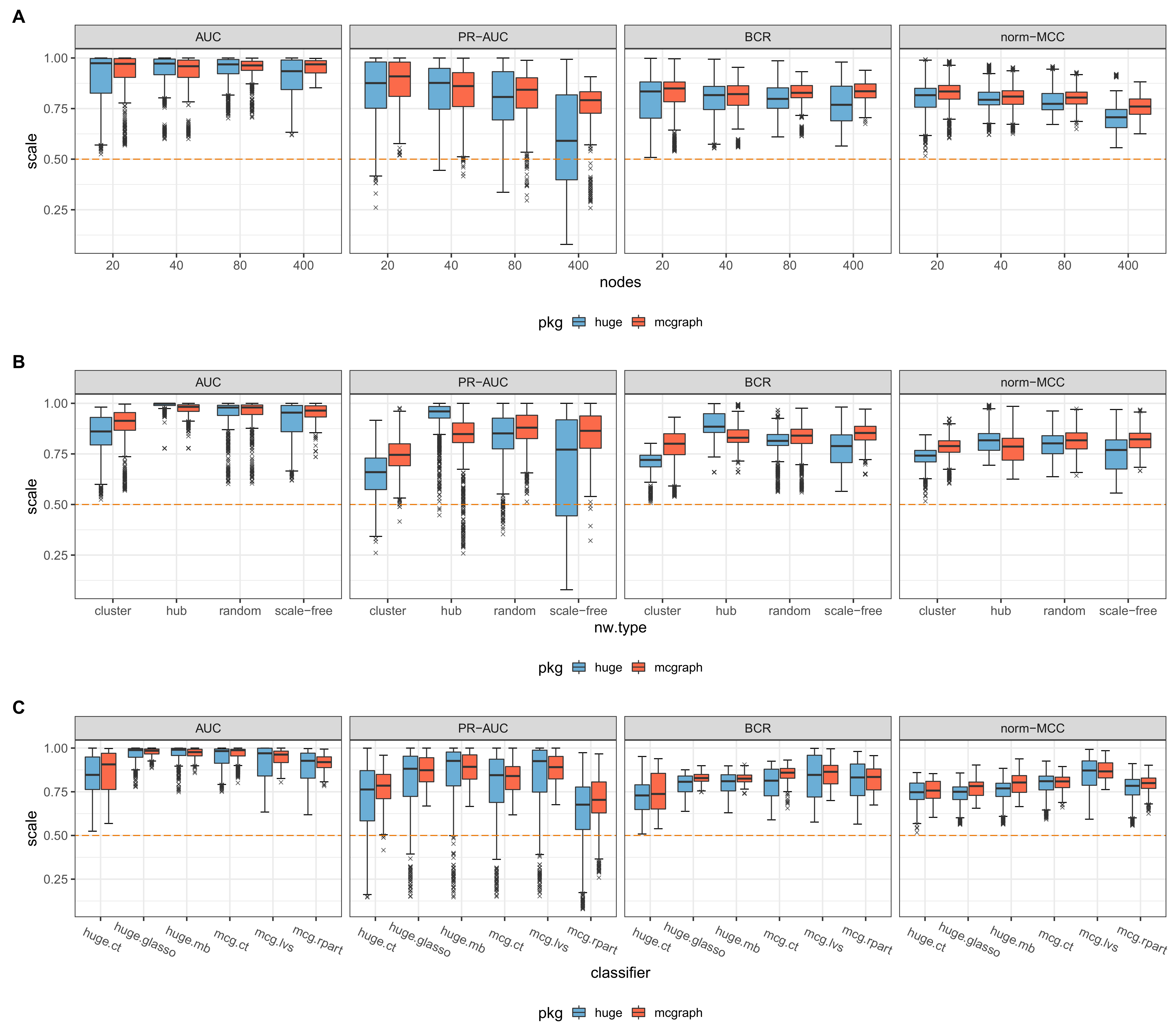
Figure 7 Comparison of prediction quality between huge and mcgraph by number of nodes,
network type and classifier. The subplot in (A) shows the results for data generated
either by huge or by mcgraph depicted as boxplots for three sets of nodes used for the
experiments: 20, 40, 80, 400. The predictions were evaluated by AUC, PR-AUC, BCR and
norm-MCC. In (B) the evaluation results are shown based on each network type: cluster,
hub, random and scale-free. (C) shows the results for each estimator function:
correlation thresholding, glasso, stability selection of huge and correlation
thresholding, forward variable selection, variable selection based on decision trees of
mcgraph. The orange dashed line indicates a random classification.
Table 3 Comparison of the overall network reconstruction quality between huge and mcgraph.
Network reconstructions were evaluated based on the means of AUC, PR-AUC, BCR and
norm-MCC for huge and mcgraph, assumed as class 1 and class 2, respectively. For each
metric Welch’s -test was performed. The table shows: mean values for both
packages, mean difference , standard error SE, upper and lower bounds for the
confidence interval of the differences
, - and -values, as well as the degrees of freedom
.
|
|
|
|
|
|
|
-value |
-value |
df |
| AUC |
0.923 |
0.939 |
-0.016 |
0.002 |
-0.020 |
-0.012 |
-8.025 |
0.000 |
7324.231 |
| PR-AUC |
0.774 |
0.823 |
-0.049 |
0.004 |
-0.056 |
-0.041 |
-12.743 |
0.000 |
6303.119 |
| BCR |
0.795 |
0.822 |
-0.028 |
0.002 |
-0.032 |
-0.024 |
-13.614 |
0.000 |
7264.842 |
| norm-MCC |
0.775 |
0.799 |
-0.024 |
0.002 |
-0.027 |
-0.021 |
-14.241 |
0.000 |
7305.602 |
We compared scores for network reconstructs based on (1) simulated data of the Monte Carlo
approach and based on (2) the data generation function of huge. Figure 7 shows box plots on the basis of number of nodes
(7A), four selected network types (7B) and six estimator functions (7C) scored by AUC,
PR-AUC, BCR and norm-MCC. Table 3 summarizes the
results after applying Welch’s -test.
Generally, we observed smaller variability concerning scores for reconstructs based on data
of mcgraph than for reconstructs based on data of huge.
This was true across all metrics. Regarding the graph types, except for the hub graph, the
median score of reconstructs based on mcgraph data was consistently higher.
For the rest, there was some variation between metrics. We observed differences between
median scores, ranges, skewness of the underlying score distributions and the number of
outliers:
| • | The AUC median score was the highest and the distribution of scores was skewed towards
higher values, as indicated by an asymmetry of upper and lower whiskers (i.e., the upper
whisker was much smaller than the lower one). In addition, the interquartile ranges
(IQRs) had a “squeezed” shape and were mostly located in the upper part of the plot.
Most reconstructs were scored best or around one, which indicates low variability. This
made comparisons across variables difficult and suggested an overly optimistic
evaluation. All AUC scores – including the lower outliers – were located above the
baseline level of a random classifier (orange dashed line). |
| • | PR-AUC scores showed the largest IQRs. The median values were lower in comparison to
AUC. While there was some tendency of skewness towards higher scores, assessing
differences in the upper range was easier when compared to AUC. Notably, very long IQRs
of the scale-free graph type and the largest graph size (400 nodes) were observed for
huge, while the results of mcgraph showed higher
median values and smaller IQRs. Some scores had values below the baseline level, implying
a more conservative evaluation of reconstructs by PR-AUC compared to AUC, as we would have
expected due to the class imbalance. |
| • | The BCR score distribution was less skewed compared to AUC and PR-AUC, as indicated by
more equal-sized whiskers. Whiskers and IQRs were generally smaller than for PR-AUC,
implying lower variability. The median scores were lower in comparison to AUC and no
score fell under the baseline level. Interestingly, while reconstructs of mcg.rpart were
scored worst by PR-AUC, regarding BCR, they were on a par with the highest scored
function mcg.lvs. |
| • | norm-MCC scores resembled scores based on BCR to a large degree: Relatively low
variability, with more equal-sized whiskers, some lower and additionally upper outliers
regarding the number of nodes and classifier functions, but no score falling below the
baseline level. |
The results after applying Welch’s t-test suggested that mean score
differences of zero were probably not compatible with scores across all metrics. Confidence
intervals suggested that lower mean values for huge compared to
mcgraph were most likely compatible with resulting scores (see Table 3).
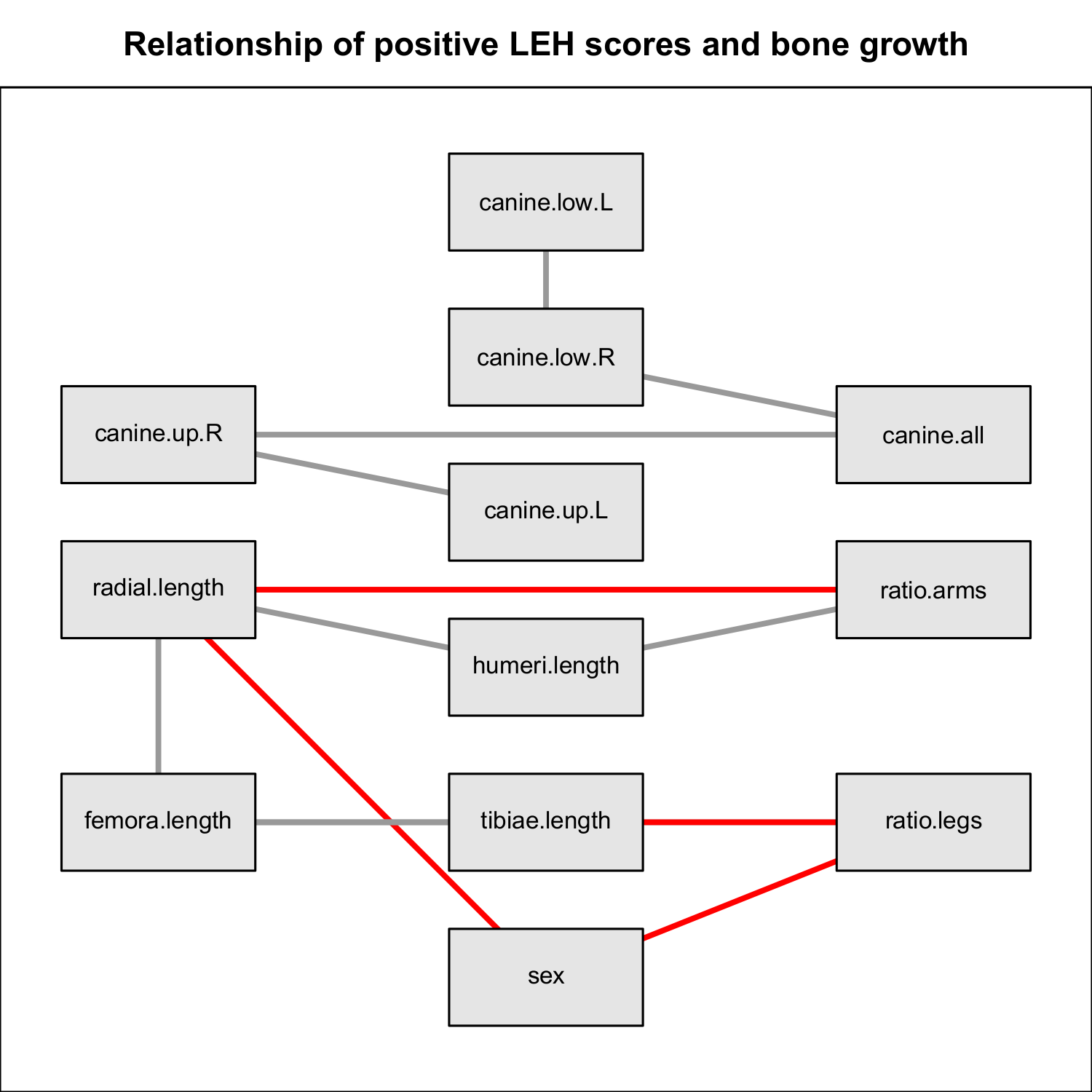
Figure 8 Network model for investigating the association between LEH in canines, bone
lengths / ratios and sex. We performed network estimation using stepwise regression
() based on a dataset of 67 medieval skeletons collected
from places in Denmark. The four canines of the upper and lower denture were given
binary scores indicating the presence of LEH (canine.up.L, canine.up.R, canine.low.L,
canine.low.R). Also, the mean for these scores has been calculated (canine.all). For the
humeri, radial bones, femora and tibiae the average length was determined
(humeri.length, radial.length, femora.length, tibiae.length), next to the ratio between
humeri and radial bones (ratio.arms) and the ratio between femora and tibiae
(ratio.legs). Additionally, the sex of the individuals is included. According to the
network model, there is no association between the LEH scores in canines and the
measures of the bones.
We applied the implementation of stepwise regression (mcg.lvs) to estimate
a network model for a real-world data set provided by Mattsson. For details see (Mattsson 2021). Figure
8 illustrates the estimated network model. There was no association of scores of
LEH in the four canines of upper and lower dentures and the anthropometric measurements of
selected bones (humeri, radial bones, thigh bones, shank bones). The LEH binary scores for
the canines were present in one component of the cluster graph, while the other component
included all variables related to measurements of the selected bones and the sex.
Discussion
We applied a simple simulation and testing framework for network reconstruction based on
data of a new Monte Carlo algorithm.
We found that network reconstructs can be improved by adjusting key parameters of the
function which generates the random data. Increasing the number of samples per variable had the largest influence on the
improvement of reconstructs. This is a consequence of general principles of Monte Carlo
sampling (Metropolis and Ulam 1949): When a
property like the association between variables is approximated, the accuracy depends on a
minimum amount of data coverage. Yet, the main advantage of randomized resampling
approaches is that this minimum is often only a small fraction of what would be needed
without iterative resampling. In our tests, 1000 samples provided optimal results. Up to date the default
sample value for the implementation in mcgraph was set to 200, which was a
compromise regarding computational cost and the quality of network reconstructs. A smaller
value of the proportion argument improved reconstructs. The argument noise
can be used to distort associations between variables by preventing correlations to develop
too quickly. As assumed prior to the test, this effect is counteracted by an increased
number of iterations. We set the default value for the number of iterations to 30 to
consider quality of reconstructs, but also the runtime of the function. We found good
default values of prop and noise to be 0.05 and 1,
respectively. A comprehensive list of arguments, default values and guidelines can be found
in Table 1 in Samples and methods.
While we concentrated on a cluster network when testing the parameters, we assumed that
results for other networks would likely resemble the previously described findings. We did a
prescreening using the simulation approach previously described for network structures with
various types and sizes. We intentionally used a network, which had scored very poorly. If
improvements based on such a poorly rated network are possible, which is the case as we
showed, it is likely that these are of general nature. The influence of the parameters can
mostly be attributed to the mechanics of the algorithm and the general principles of the
Monte Carlo method as a randomized stochastic process (e.g., more samples = better coverage
= better approximation).
The comparative analysis of the Monte Carlo simulated data showed higher mean scores for
reconstructs based on mcgraph compared to huge in support
of our general hypothesis. AUC scores (,
, ) can be assumed to be biased upwards due to strong negative
skewness of the score distribution (see figure 7). As mentioned earlier, AUC is unsuitable
for an imbalanced classification set. Scores of PR-AUC (
) were considerably lower, reflecting a more conservative
evaluation, but the variability of the individual scores was much higher compared to the
other metrics especially for huge data. While it is better suited for class
imbalance (Saito and Rehmsmeier 2015), its
valuation scheme is a function of the degree of imbalance (i.e., a graph’s sparsity).
Consequently, scores are accurate for large class imbalances, but for smaller imbalances the
scores should be corrected downwards (Boyd et al.
2012). We did not apply this correction in our study, and it would not change the
implications of our main findings, because we concentrated on mean differences between the
packages. Still, this should be considered for any follow-up analysis. BCR scores
(
) showed relatively low variability of individual scores. The
same was true for norm-MCC (
). The mean scores of the latter were the most conservative.
MCC is a total summary score of all outcomes and provides a balanced assessment of the
relation of FP and FN. Chicco and Jurman note, that it is mostly the best metric to use,
especially in case of class imbalance (Chicco and Jurman
2020).
The results additionally showed that network reconstructs for scale-free networks based on
Monte Carlo data were especially well assessed. This is noteworthy, because networks of
cells, social relationships or other real-world systems are often characterized by such a
structure (Barabási and Oltvai 2004). These networks
are not fixed concerning their size, but dynamically grow by preferential attachment (i.e.,
nodes connect to already high-degree nodes) so that they are characterized by a power-law
degree distribution (Barabási 1999; Barabási and Pósfai 2016).
Concerning the relationship of LEH scores and bone growth, we did not find any association.
The generated network estimate after stepwise regression showed a cluster graph with two
separate components, one component containing all bone related variables and the other one
contained all variables related to LEH scores of canines. By and large, this result agreed
with the more extensive statistical analysis done by (Mattsson 2021), where SNHA was applied.
Throughout our analysis we used a version of stepwise regression and we have already noted,
that this method is problematic. We still used it because (1) in our network reconstruction
analysis the true model was known beforehand or in the case of the LEH model, there was at
least some model by another method / study we could compare our results with, (2) we also
applied a collection of alternative methods in comparison and (3) it seemed, that our
implementation based on preselecting covariates by highest correlation, using AIC and
improved empirical results. But this might not help with
the fundamental issues, that variables are selected one after another purely based on the
underlying data using statistics, which are meant to be applied on prespecified models
(Harrell 2001). Thus, despite appearing as a
straightforward approach stepwise selection must be used very carefully or should better be
replaced with alternative methods (Huberty 1989;
Heinze and Dunkler 2017; Smith 2018).
Another possible limitation of our analysis is the use of classification: Classification
reduces the degree of information of a signal by binarization, reframing the initial problem
as an either-or question. F. E. Harrell notes, that in many circumstances this is not the
right way to confront real-world problems and argues for the use of probabilistic model
approaches and methods based on bootstrapping instead (Harrell 2001).
The last step of our testing
framework must not necessarily be based on classification, as we did here, but might well be
based on a richer probabilistic approach, where the presence of associations is modeled by
probabilities or on bootstrapping to assign empirical confidence intervals for each edge.
The important point is that there is a pre-defined structure at hand and suitable randomized
data based on it to begin with. Overall, the analysis of synthetic networks can be
worthwhile, and our Monte Carlo approach has the advantage of being conceptually and
practically simple but extendable. It offers the possibility to use (weighted) un- and
directed input graphs for simulation analysis and generates suitable data for it.
Conclusion
Generating synthetic data for graphs and evaluate network reconstructs of methods of
interest, can be one step in the process of method verification by researchers. The
mcgraph R package offers various features to create and plot graph structures, as
well as to generate synthetic data based on given graph structures for the purpose of
network reconstruction. The simple Monte Carlo algorithm presented in this paper generates
simulated data with quality at least as good as the comparable R package
huge for cluster, random, hub and scale-free network types of various sizes.
By adjusting a small set of parameters, like the number of samples generated per node the
data can be further optimized. The package is currently submitted to the “The Comprehensive
R Archive Network” and should be available soon as an official R
package.
List of Abbreviations
| Abbreviations |
Meaning |
| ADBOU |
Anthropological DataBase Odense University |
| AIC |
Akaikes Information
Criterion |
| AUC |
Area Under the Receiver Operating
Characteristic Curve |
| BCR |
Balance Classification
Rate |
| CI95% |
95% Confidence
Interval |
| FN |
False Negative |
| FP |
False Positive |
| FPR |
False Positive Rate |
| IQR |
InterQuartile Range |
| LEH |
Linear Enamel
Hypoplasia |
| MCC |
Matthews Correlation
Coefficient |
| norm-MCC |
nomalized Matthews Correlation
Coefficient |
| PPV |
Positive Predictive
Value |
| PR-AUC |
Area Under the Precision Recall
Curve |
| PRC |
Precision Recall
Curve |
| ROC |
Receiver Operating Characteristic
Curve |
| SNHA |
St. Nicolas House
Analysis |
| TN |
True Negative |
| TNR |
True Negative Rate or
specificity |
| TP |
True Positive |
| TPR |
True Positive Rate, sensitivity or
recall |
Appendix
Table 2 List of arguments and guidelines for parameters of the Monte Carlo algorithm.
Argument, description with guidelines and default values of the Monte Carlo algorithm
implemented in the R package mcgraph (Groth and
Novine 2022).
| Argument |
Description |
Default |
| A |
Input graph. This can be a (weighted) directed or undirected graph, given as an
adjacency matrix. |
- |
| n |
The number of generated data values for each variable. The initial values are
drawn from a normal distribution as described before. More values should lead to
pronounced correlations and better reconstructs but will increase the runtime and
memory allocation. |
200 |
| iter |
The number of iterations, (i.e., the steps of refinement of the data). In each
iteration the values of outgoing neighboring nodes become more and more similar.
This argument counteracts noise
(i.e., more iteration steps should decrease the influence of
noise and allow for more
pronounced correlations but only to an upper bound). |
30 |
| val |
The given mean value of the normal distribution the random values are drawn
from. The default value of 100 is chosen based on practical considerations:
noise, which is added after
each iteration and drawn from a normal distribution with a mean of 0, should only
be a small fraction of the data values. |
100 |
| sd |
The given value for the standard deviation of the normal distribution the random
values are drawn from. The default value of 2 is chosen to allow for a
sufficiently large spread of the initial values. |
2 |
| prop |
The proportion, which determines how the values of the respective source and
target node are weighted when calculating the updated value of the target in each
iteration. Larger values increase the weighting of the source and decrease the
weighting of the target for the calculation of the weighted mean. |
0.05 |
| noise |
The level of random noise, which is added to the data values in each iteration
step. It indicates the value for the standard deviation of a normal distribution
with mean 0 from which values are drawn randomly. The influence of
noise is dependent on
val (i.e., higher values for
noise will lead to less
pronounced correlations between variables). We use a normal distribution with mean
0 to let noise only be small
fraction of val. This can be
counterbalanced by increasing the value for
iter. |
1 |
| init |
An optional argument to prespecify an alternative set of starting data. |
NULL |
References
Akaike, H. (1974). A new look at the statistical
model identification. IEEE Transactions on Automatic Control 19 (6), 716–723. https://doi.org/10.1109/TAC.1974.1100705.
Barabási, A.-L. (1999). Emergence of scaling in
random networks. Science 286 (5439), 509–512. https://doi.org/10.1126/science.286.5439.509.
Barabási, A.-L. (2007). Network medicine – from
obesity to the "Diseasome". The New England Journal of Medicine 357 (4), 404–407.
https://doi.org/10.1056/NEJMe078114.
Barabási, A.-L./Gulbahce, N./Loscalzo, J. (2011).
Network medicine: a network-based approach to human disease. Nature Reviews Genetics 12
(1), 56–68. https://doi.org/10.1038/nrg2918.
Barabási, A.-L./Oltvai, Z. N. (2004). Network
biology: understanding the cell's functional organization. Nature Reviews Genetics 5
(2), 101–113. https://doi.org/10.1038/nrg1272.
Barabási, A.-L./Pósfai, M. (2016). Network
science. Cambridge, Cambridge University Press.
Batushansky, A./Toubiana, D./Fait, A. (2016).
Correlation-Based Network Generation, Visualization, and Analysis as a Powerful Tool in
Biological Studies: A Case Study in Cancer Cell Metabolism. BioMed Research
International 2016, 8313272. https://doi.org/10.1155/2016/8313272.
Berrar, D./Granzow, M./Dubitzky, W. (2007).
Fundamentals of data mining in genomics and proteomics. Boston, MA, Springer; Springer
US.
Boyd, K./Santos Costa, V./Davis, J./Page, C. D.
(2012). Unachievable region in precision-recall space and its effect on empirical
evaluation. In: J. Langford/J. Pineau (Eds.). Proceedings of the 29th International
Conference on Machine Learning // Proceedings of the Twenty-Ninth International
Conference on Machine Learning. Edinburgh, [International Machine Learning Society],
1616–1626.
Breiman, L./Friedman, J. H./Olshen, R. A./Stone,
C. J. (1984). Classification and regression trees. Belmont, Calif.,
Wadsworth.
Büttner, K./Salau, J./Krieter, J. (2016). Adaption
of the temporal correlation coefficient calculation for temporal networks (applied to a
real-world pig trade network). SpringerPlus 5, 165. https://doi.org/10.1186/s40064-016-1811-7.
Cao, C./Chicco, D./Hoffman, M. M. (2020). The
MCC-F1 curve: a performance evaluation technique for binary classification. https://doi.org/10.48550/arXiv.2006.11278.
Chicco, D./Jurman, G. (2020). The advantages of
the Matthews correlation coefficient (MCC) over F1 score and accuracy in binary
classification evaluation. BMC Genomics 21 (1), 6. https://doi.org/10.1186/s12864-019-6413-7.
Christakis, N. A./Fowler, J. H. (2007). The spread
of obesity in a large social network over 32 years. New England Journal of Medicine 357
(4), 370–379. https://doi.org/10.1056/NEJMsa066082.
Copas, J. B./Long, T. (1991). Estimating the
residual variance in orthogonal regression with variable selection. The Statistician 40
(1), 51–59. https://doi.org/10.2307/2348223.
Dahl, D. B./Scott, D./Roosen, C./Magnusson,
A./Swinton, J. (2000). xtable: Export Tables to LaTeX or HTML. Available online at
https://CRAN.R-project.org/package=xtable (accessed
5/31/2022).
Eddelbuettel, D./François, R. (2011). Rcpp:
Seamless R and C++ integration. Journal of Statistical Software 40 (8), 1–18. https://doi.org/10.18637/jss.v040.i08.
Eddelbuettel, D./Sanderson, C. (2014).
RcppArmadillo: Accelerating R with high-performance C++ linear algebra. Computational
Statistics and Data Analysis 71, 1054–1063. https://doi.org/10.1016/j.csda.2013.02.005.
Efron, B./Tibshirani, R. (1986). Bootstrap methods
for standard errors, confidence intervals, and other measures of statistical accuracy.
Statistical Science 1 (1), 54–75. https://doi.org/10.1214/ss/1177013815.
Frayling, T. M./Timpson, N. J./Weedon, M.
N./Zeggini, E./Freathy, R. M./Lindgren, C. M./Perry, J. R. B./Elliott, K. S./Lango,
H./Rayner, N. W./Shields, B./Harries, L. W./Barrett, J. C./Ellard, S./Groves, C.
J./Knight, B./Patch, A./Ness, A. R./Ebrahim, S./Lawlor, D. A./Ring, S. M./Ben-Shlomo,
Y./Jarvelin, M.-R./Sovio, U./Bennett, A. J./Melzer, D./Ferrucci, L./Loos, R. J.
F./Barroso, I./Wareham, N. J./Karpe, F./Owen, K. R./Cardon, L. R./Walker, M./Hitman, G.
A./Palmer, C. N. A./Doney, A. S. F./Morris, A. D./Smith, G. Davey/Hattersley, A.
T./McCarthy, M. I. (2007). A common variant in the FTO gene is associated with body mass
index and predisposes to childhood and adult obesity. Science 316 (5826), 889–8894.
https://doi.org/10.1126/science.1141634.
Friedman, J./Hastie, T./Tibshirani, R. (2008).
Sparse inverse covariance estimation with the graphical lasso. Biostatistics 9 (3),
432–441. https://doi.org/10.1093/biostatistics/kxm045.
Ghazalpour, A./Doss, S./Zhang, B./Wang,
S./Plaisier, C./Castellanos, R./Brozell, A./Schadt, E. E./Drake, T. A./Lusis, A.
J./Horvath, S. (2006). Integrating genetic and network analysis to characterize genes
related to mouse weight. PLOS 2 (8), 1182–1192. https://doi.org/10.1371/journal.pgen.0020130.
Groth, D./Novine, M. (2022). mcgraph. Available
online at https://github.com/MasiarNovine/mcgraph (accessed
1/18/2022).
Groth, D./Scheffler, C./Hermanussen, M. (2019).
Body height in stunted Indonesian children depends directly on parental education and
not via a nutrition mediated pathway - Evidence from tracing association chains by St.
Nicolas House Analysis. Anthropologischer Anzeiger 76 (5), 445–451. https://doi.org/10.1127/anthranz/2019/1027.
Hanley, J. A./McNeil, B. J. (1982). The meaning
and use of the area under a receiver operating characteristic (ROC) curve. Radiology 143
(1), 29–36. https://doi.org/10.1148/radiology.143.1.7063747.
Harrell, F. E. (2001). Regression modeling
strategies - with applications to linear models, logistic regression, and survival
analysis. 2nd ed. New York, Springer.
Heinze, G./Dunkler, D. (2017). Five myths about
variable selection. Transplant International 30 (1), 6–10. https://doi.org/10.1111/tri.12895.
Heinze, G./Wallisch, C./Dunkler, D. (2018).
Variable selection - A review and recommendations for the practicing statistician.
Biometrical Journal 60 (3), 431–449. https://doi.org/10.1002/bimj.201700067.
Hermanussen, M./Aßmann, C./Groth, D. (2021). Chain
reversion for detecting associations in interacting variables - St. Nicolas house
analysis. International journal of environmental research and public health 18 (4),
1741. https://doi.org/10.3390/ijerph18041741.
Huberty, C. J. (1989). Problems with stepwise
methods – better alternatives. Advances in Social Science Methodology (1),
43–70.
Jiang, H./Fei, X./Liu, H./Roeder, K./Lafferty,
J./Wasserman, L./Li, X./Zhao, T. (2021). High-dimensional undirected graph estimation.
Available online at https://cran.r-project.org/web/packages/huge/huge.pdf (accessed
1/18/2022).
Langfelder, P./Horvath, S. (2008). WGCNA: an R
package for weighted correlation network analysis. BMC Bioinformatics 9, 559. https://doi.org/10.1186/1471-2105-9-559.
Loscalzo, J./Barabási, A.-L./Silverman, E. (2017).
Network medicine: Complex systems in human disease and therapeutics. Cambridge, Harvard
University Press.
Matthews, B. W. (1975). Comparison of the
predicted and observed secondary structure of T4 phage lysozyme. Biochimica et
Biophysica Acta (BBA) - Protein Structure 405 (2), 442–451. https://doi.org/10.1016/0005-2795(75)90109-9.
Mattsson, C. C. (2021). Correlation between childhood episodes of stress and long bone-ratios
in samples of medieval skeletons - using linear enamel hypoplasia as proxy. Human Biology and Public Health 3. https://doi.org/10.52905/hbph2021.3.23.
Meinshausen, N./Bühlmann, P. (2006).
High-dimensional graphs and variable selection with the Lasso. The Annals of Statistics
34 (3), 1436–1462. https://doi.org/10.1214/009053606000000281.
Meinshausen, N./Bühlmann, P. (2010). Stability
selection. Journal of the Royal Statistical Society. Series B, Statistical Methodology
72 (4), 417–473. https://doi.org/10.1111/j.1467-9868.2010.00740.x.
Metropolis, N./Ulam, S. (1949). The Monte Carlo
method. Journal of the American Statistical Association 44 (247), 335–341. https://doi.org/10.2307/2280232.
Milner, G. R./Boldsen, J. L. (2012). Transition
analysis: a validation study with known-age modern American skeletons. American Journal
of Physical Anthropology 148 (1), 98–110. https://doi.org/10.1002/ajpa.22047.
Nicosia, V./Tang, J./Mascolo, C./Musolesi,
M./Russo, G./Latora, V. (2013). Graph metrics for temporal networks. In: P. Holme/J.
Saramäki (Eds.). Temporal networks. Petter Holme; Jari Saramäki, eds. Heidelberg,
Springer, 15–40.
R Core Team (2021). R: a language and environment
for statistical computing. R Foundation for Statistical Computing. Available online at
https://www.r-project.org/.
Rice, J. J./Tu, Y./Stolovitzky, G. (2005).
Reconstructing biological networks using conditional correlation analysis.
Bioinformatics 21 (6), 765–773. https://doi.org/10.1093/bioinformatics/bti064.
Saito, T./Rehmsmeier, M. (2015). The
precision-recall plot is more informative than the ROC plot when evaluating binary
classifiers on imbalanced datasets. PLOS ONE 10 (3), 1–21. https://doi.org/10.1371/journal.pone.0118432.
Sakamoto, Y./Ishiguro, M./Kittagawa, G. (1986).
Akaike information criterion statistics. Dordrecht, Reidel.
Sanderson, C./Curtin, R. (2016). Armadillo: a
template-based C++ library for linear algebra. Journal of Open Source Software 1 (2),
26. https://doi.org/10.21105/joss.00026.
Sanderson, Conrad/Curtin, Ryan (2018). A
user-friendly hybrid sparse matrix class in C++. In: J. H. Davenport/M. Kauers/G. Labahn
et al. (Eds.). Mathematical Software – ICMS 2018. 6th International Conference, South
Bend, IN, USA, July 24-27, 2018, Proceedings. Cham, Springer International Publishing,
422–430.
Smith, G. (2018). Step away from stepwise. Journal
of Big Data 5 (1), 32. https://doi.org/10.1186/s40537-018-0143-6.
Sulaimanov, N./Koeppl, H. (2016). Graph
reconstruction using covariance-based methods. EURASIP Journal on Bioinformatics and
Systems 19 // 2016 (1), 267–288. https://doi.org/10.1186/s13637-016-0052-y.
Tarp, P. (2017). Skeletal age estimation: a
demographic study of the population of Ribe through 1000 years. Ph.D. dissertation.
Odense, Syddansk Universitet.
Wasserman, L. (2013). All of statistics: a concise
course in statistical inference. A concise course in statistical inference. New York,
Springer.
Wasserman, S./Faust, K. (1994). Social network
analysis: methods and applications. Cambridge, Cambridge University
Press.
Wickham, H. (2016). ggplot2: elegant graphics for
data analysis. 2nd ed. Cham, Springer.
Xie, Y. (2021). knitr: A General-purpose package
for dynamic report generation in R. Available online at https://yihui.org/knitr/.
Zhang, B./Horvath, S. (2005). A general framework
for weighted gene co-expression network analysis. Statistical Applications in Genetics
and Molecular Biology 4, 17. https://doi.org/10.2202/1544-6115.1128.
Zhao, T./Liu, H./Roeder, K./Lafferty,
J./Wasserman, L. (2012). The huge package for high-dimensional undirected graph
estimation in R. Journal of Machine Learning Research 13, 1059–1062.