Contents

Introduction

In the first part of this review series (Groth 2024), I covered the basics of research types (e.g., correlational versus experimental research, the foundations of representative sampling, the problems associated with it, and how to determine the data types of our variables and their representation within data structures using the R programming language. I also explained why using a programming language like R is preferable to using spreadsheet software. The main benefit of using a tool such as R (R Core Team 2025), Python (Python Core Team 2025), or Octave (Bateman et al. 2025) for statistics, is that it separates data and analysis into different files. This simplifies reusing the analysis steps with new or changed data.

The second part of this series will focus on univariate statistics and associated terminology, such as descriptive and inferential statistics, p-values, confidence intervals, and effect size measures. First, we will review the terminology, and then we will apply it to univariate statistical problems. Finally, we will provide basic sample code demonstrating how to perform such analyses using the R programming language.

Descriptive and Inferential Statistics

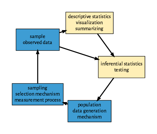
The objective of descriptive statistics is to summarize the observed data (often some sample data) and visualize trends, thereby improving understanding of the data. Then, in inferential statistics, we draw conclusions about the likelihood of estimates obtained from the observed data in relation to assumed properties of the underlying population or data generating mechanism. For example, data observed on one group may have values that are, on average, higher than those observed for the other group. However, we want to conclude that these differences are significant and not just due to chance. Inferential statistics typically uses statistical tests incorporating the assumed properties of the population. In this part of the analysis, we try to generalize our findings. The full process is visualized in Fig. 1. Other types of statistical analysis determine the strength of associations, or correlations, between two or more variables, and for the case of a few or many interacting variables, visualize these correlations in network-like structures. Other types of statistics deal with grouping of items, such as clustering, which is an unsupervised learning approach. Methods that predict the outcome of one or more variables based on one or more others are also called supervised learning or modeling methods. Supervised and unsupervised learning methods belong to the field of machine learning. These methods will be covered in later parts of this review series.

Figure 1  The role of descriptive and inferential statistics. A representative sample, the observed data, is drawn from the population using a data generation mechanism like a survey or some measurements (bottom) through an unbiased selection mechanism, sampling (left). Descriptive statistics (top) work with the sample data, summarizing and visualizing it with plots. Inferential statistics (right) then allows to draw conclusions about the population, a process called generalization.

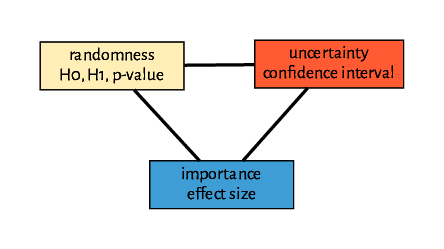
Figure 2  The role of p-values, confidence intervals, and effect sizes. A p-value only states the probability of getting a result in our sample with such a difference, or a larger one. It expresses the randomness of our result. A confidence interval describes where we believe the population parameter lies. Finally, the effect size allows us to communicate the size of a difference, such as between groups or between a sample and the population.

Confidence Intervals

Before discussing the basics of univariate statistics, we will review a few statistical terms (Fig. 2). First, we will elaborate on the term “confidence interval”. When we sample from a population, i.e., we consider a data generating mechanism. For example, when we collect body height values from bioinformatics students in Germany - we are interested in knowing the average body height of all bioinformatics students. In principle, however, we cannot answer this question because we only have a sample of bioinformatics students in Germany. Therefore, we cannot determine the population value, also called the population parameter or parameter of the data generating mechanism. However, based on our sample, we can express a range within which the population parameter is likely to fall with a specific degree of certainty. Typically, a range with 95% certainty is used. This range of values is called the confidence interval. The 95% confidence interval is the range in which the assumed population parameter is likely to fall 95% of the time, this means that, on average, in five out of 100 times, the confidence interval reported in scientific articles, or which we get in our own R analysis, will not contain the assumed population parameter. It is impossible to know the population parameter by using a sample alone. To do so, we would need to observed (“sample”) the entire population.

Survey Example Data Set

To illustrate, let’s use the survey dataset from the Table 1 to learn more about the main variables.

The main purpose of this data collection is to provide examples of different types of statistical procedures, plots, tests, etc. using well-understood data as the students work with their own data. For example, the dataset allows you to answer questions such as “Do feel people luckier if they are male?”, or “Do people born in spring and summer feel luckier than people born in seasons with less sunlight?” (Chotai and Wiseman 2005), or “Are students taller than the average population?”. The main goal of this dataset is to focus on statistical rather than biological questions. Working with their own data usually motivates students to pay closer attention to the lecturer.

Confidence Interval of a Proportion

Let’s determine the proportion of students attending a master’s degree program who smoke and who are studying life sciences or bioinformatics. The R code in Listing 1 imports the survey data from two master’s programs into a data frame and then calculates the proportion of smokers.

survey=read.table("data/survey-2021-11.tab",header=TRUE,
stringsAsFactors=TRUE)
colnames(survey)[1]="sex" # rename a column
dim(survey) # check row and column number
### [1] 617 10
head(survey[,1:6]) # display first 6 rows
### sex cm kg ssize smoker meat
### 1 F 163 62.5 38 N 3
### 2 M 180 80.0 43 Y 5
### 3 F 158 52.0 37 N 2
### 4 F 179 79.0 42 Y 3
### 5 M NA 80.0 NA N 1
### 6 M 188 85.0 44 N 1
table(survey$smoker,useNA="ifany") # check number of (non-)smokers
###
### N Y <NA>
### 540 74 3
prop.table(table(survey$smoker)) # calculate proportions
###
### N Y
### 0.8794788 0.1205212
prop.test(table(survey$smoker)) # test 50/50 (default)
###
### 1-sample proportions test with continuity correction
###
### data: table(survey$smoker), null probability 0.5
### X-squared = 352.16, df = 1, p-value < 2.2e-16
### alternative hypothesis: true p is not equal to 0.5
### 95 percent confidence interval:
### 0.8504564 0.9036343
### sample estimates:
### p
### 0.8794788
p=0.8795
p - 1.96 * sqrt((p * (1-p) ) / (540+74)) # lower CI bound approximated
### [1] 0.8537496

Let’s assume that the students in our sample are representative of all Master’s students studying life sciences in Germany. Around 12% of the students in our sample are smokers, and around 88% are nonsmokers (Fig. 3). These are the values for our sample. But what are the values in the population? Since we cannot determine this value via a complete population census, we provide a range reflecting our assumption regarding the data generating mechanism, i.e., the population, with 95% percent confidence. For nonsmoking students, the range is 85-90%, and for smoking students, it is 10-15%. The confidence interval (CI) can be determined for large sample sizes based on the asymptotic properties of the test statistic, i.e., the proportion, using the following simple formula

This formula should not be used if the number of observations (N) is less than 10. The number of positive hits (the enumerator) must also be greater than or equal to 5. When these thresholds are not met, the confidence intervals can be derived based on the binomial distribution.

Confidence Interval for a Mean

As for proportions, we can determine the confidence interval also for the mean. For example, we will calculate the mean body height of students in my biostatistics courses. In principle, it is expected that students are taller than the general population (Arntsen et al. 2023). However, it does not make sense to measure the average body height without separating the students by their sex, as women are, on average, around 12 cm shorter than men. We separate the two levels of these variables using R’s aggregate function and then provide the qualitative variable, here sex, and the function we would like to apply (Listing 2).

The range of these values indicates the range within which we are 95% confident that the true parameter lies. On average, a reported confidence interval contains the true population parameter 95 out of 100 times. In 5% of cases where we read a confidence interval in the literature, the interval does not contain the true population parameter.

aggregate(survey$cm,by=list(survey$sex),mean, na.rm=TRUE)
### Group.1 x
### 1 F 167.3274
### 2 M 180.3961
aggregate(survey$cm,by=list(survey$sex),function (x) t.test(x)$conf.int)
### Group.1 x.1 x.2
### 1 F 166.6402 168.0147
### 2 M 179.3827 181.4095

P-values

Confidence intervals express the range in which the true value of a population parameter is believed to lie. P-values, on the other hand, express the maximum probability of obtaining a result by chance (Sil et al. 2019). The p-value is related to the so-called “null hypothesis” (H0), which suggests that there is no effect or relationship between the variables. Since we are often interested in the opposite, there is usually an alternative hypothesis (H1) that assumes a relationship. If the p-value is very low, usually below 0.05, we reject the null hypothesis and we accept the alternative hypothesis.

In principle, low p-values indicate that it is unlikely to get such a result if the two groups do not vary with regard to our variable of interest. In our example above for the number of smokers, we can see that the p-value is less than 2.2e-16, a very low value, so it is highly unlikely that the difference in the number of smoking and nonsmoking students occurred by chance. In this context, the p-value expresses the randomness of our result. The exact value depends greatly on the sample size. With larger sample sizes the p-value can quickly become very low, even for small differences between two groups.

Since the p-value only indicates the probability of obtaining such a result, it is common practice to not focus on the exact value, but rather to present it at three different levels of significance, p less than .05$p<.05$ (called “significant”), p less than .01$p<.01$ (called “highly significant”) and p less than .001$p<.001$ (called “extremely significant”). In a statistical sense, the term “significant” should not be interpreted as “important”, as it is merely a measure of probability and thus expresses some degree of randomness in the result. An alternative to presenting the p-value as a numeric value is to use one asterisk for p less than .05$p<.05$, two forp less than .01$p<.01$ or three for p less than .001$p<.001$.

Effect Sizes

Since, in addition to the p-value, the confidence intervals are often reported, the same is not usually done for effect sizes in the literature. This is a significant omission in the communication of a result. Instead of focusing on the significance level with the p-value you should focus on the effect size. For example, drug researchers might communicate the number needed to treat (NNT) to avoid one case of hospitalization or death, as this clearly communicates the benefits and costs of a drug in terms of health improvements, financial costs, and possible unwanted side effects. Depending on the data type, different effect size measures exist. They are usually dimensionless, meaning they do not depend on the measurement scale. This allows for the comparison of different variables.

Common effect size measures for problems of univariate and bivariate statistics for qualitative data include, for example Cohen’s w or the odds ratio (Tab.2). For numerical data, the common measure is Cohen’s d, which is the difference in means between two groups or the sample and the population divided by the standard deviation. The strength of the association between two numerical variables is expressed by a correlation coefficient, such as Pearson’s r or Spearman’s rho.

Univariate Statistics

Univariate statistics usually compare a sample against a known population parameter, for quantitative data, this is usually the mean, for qualitative data, it is often the proportion. To test for significant differences, One Sample tests are performed at the end. Examples for these analyses using the survey data set described above might include comparing whether students of these biological topics are taller than the average population or whether these students smoke less than the general population in Germany.

We can distinguish different analysis steps in statistics:

descriptive statistics:

inferential statistics:

N stands here for numerical data, C for qualitative/ categorical data.

Quantitative data

Quantitative data analysis relies on statistical measures and procedures to summarise the data distributions, create visualizations, test hypotheses and quantify effects. To summarise the center of the distribution, the mean (the arithmetic average) and the median (the middle value), and the mode are usually used. Whereas the mean is sensitive to outliers, the median is robust against outliers and skewed distributions. To describe the data dispersion, the standard deviation (the square root of the variance) is usually used. It can be seen as the approximate average distance from the mean of the values. Higher values of the standard deviation (s) indicate greater dispersion of the data.

The formula is

Where x is the sample mean and xi are the sample values.

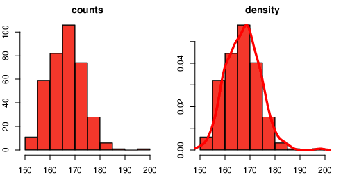
Visualizations of univariate numerical data are usually done using a histogram containing frequency bins of the data. Often a density line is layered on top of them. The latter are smoothed probability curves expressing the data trend. Let’s demonstrate this with some R code for analyzing women’s height data of our survey data (Listing 3):

fsurvey=survey[survey$sex=="F",] ## extract female data
mean(fsurvey$cm,na.rm=TRUE)
### [1] 167.3274
median(fsurvey$cm,na.rm=TRUE)
### [1] 168
sd(fsurvey$cm,na.rm=TRUE)
### [1] 6.704708
png("fhist.png",width=700,height=350) ## start the plot
par(mfrow=c(1,2),mai=rep(0.4,4)) ## multifigure setup
hist(fsurvey$cm,col="salmon",main="counts")
hist(fsurvey$cm,freq=FALSE,col="salmon",main="density")
lines(density(fsurvey$cm,na.rm=TRUE),lwd=4,col="red")
dev.off() ## end the plot

Figure 3  R-code output for visualization of numerical data. On the left, a histogram of the frequency distribution of the body height of female students is shown. On the right a density line is layered over these frequency bars using the lines function of R.

To test the null hypothesis (H0), that the sample and the population have the same distribution characteristics, the sample data and the known population parameter can be used to perform an One Sample t-test for normally distributed data. If the data are not normally distributed, a Wilcoxon signed-rank should be used instead. The t-value for the t-test is determined as follows:

where x is the sample mean, mu$\mathit{\mu }$ the population parameter, s the sample standard deviation and N the sample size.

The Wilcoxon signed-rank test ranks the differences between the population mean and the values of our sample and then compares the summed ranks with a null distribution where on average half of the values should be smaller, and half of the values larger than the population mean. If the p-value is less than 0.05, the null hypothesis is rejected in favor of the alternative hypothesis that the data for both groups are different.

If the result is significant, it makes sense to calculate the effect size. This can be quantified using Cohen’s d formula:

mu$\mathit{\mu }$ is the population mean, x is the sample mean, and s$s$ the standard deviation. If we compare two groups, Cohen’s d is then the difference by the means of the two groups divided by the pooled standard deviation of both groups, so it is then just the difference of the two means in relation to the spread of the data. Cohen’s rule of thumb (Cohen 1992), states that values of around 0.2, 0.5, and 0.8 represent small, medium, and large effects, respectively.

Listing 4 shows the R-code and the results of our analysis:

shapiro.test(fsurvey$cm) # check for normality p<.05 not normal
###
### Shapiro-Wilk normality test
###
### data: fsurvey$cm
### W = 0.98797, p-value = 0.003898
t.test(fsurvey$cm,mu=165) # test for normal data (as we have large N)
###
### One Sample t-test
###
### data: fsurvey$cm
### t = 6.6592, df = 367, p-value = 1.007e-10
### alternative hypothesis: true mean is not equal to 165
### 95 percent confidence interval:
### 166.6402 168.0147
### sample estimates:
### mean of x
### 167.3274
wilcox.test(fsurvey$cm,mu=165) # as data are not normal
###
### Wilcoxon signed rank test with continuity correction
###
### data: fsurvey$cm
### V = 41218, p-value = 8.034e-10
### alternative hypothesis: true location is not equal to 165
library(sbi) # load the sbi library
sbi$cohensD(fsurvey$cm,mu=165) # effect size
### [1] -0.347136

The statistical analysis should usually close with a test report that states the problem, the main statistics, the test result, and the effect size as shown below:

In our study we compared the average body height of female students with that of females of the same age class in the general population.

An One Sample t-test revealed that our female students of our Master courses are significantly taller (mean=167.3cm, s=6.7, CI95%=[166.6,168.0], t=6.7(df=367), p less than .001$p<.001$, d=0.35) than females of the general population (165cm) The Wilcoxon test corroborated this finding (V=41218, p less than .001$p<.001$), confirming taller body height of our students.

If the data are not normally distributed and the sample size is smaller, let’s say less than 50 samples, only the Wilcoxon test should be performed.

Qualitative Data

Let’s continue with the univariate analysis of qualitative (categorical) data which involves summarizing the distribution of a single variable using frequency-based measures and visualizations. In this context, the mode is the key descriptive statistic for categorical data, representing the category with the highest frequency or count. In our survey data, for example, the ‘non-smoker category is assigned more often than the ’smoker’ category, so the mode is ‘non-smoker’.

As well as using the mode, we can express the fractions of the different categories as proportions or percentages (i.e., proportions multiplied by 100) to provide a clear data summary. These results are typically presented in tables that list each category as a count, proportion, or percentage.

Bar plots (also called bar charts) are typically used as visualizations for qualitative data. These display the frequencies as separate bars, making it easy to compare the categories. An alternative are Dot plots, which represent each observation as a dot. These are often useful if a second variable should be added to the same plot. Pie charts show the frequencies as slices of a circle. However, as people often have difficulty determining angles visually, bar plots or dot plots are generally preferred for their clarity.

In inferential statistics, the one-sample proportion test can be used to determine whether the observed proportion in a sample differs significantly from a hypothesized or known population proportion. This test involves formulating a null hypothesis (e.g., that sample proportion is equal to the population proportion) and calculating a test statistic based on the observed proportion, the hypothesized value, and the sample size. This approach is most suitable when data are randomly sampled and follow a binomial distribution, and it is particularly reliable with larger samples.

Cohen’s w is used to quantify the magnitude of any observed difference and is an effect size measure for proportions and categorical data. It is calculated as the square root of the sum of squared differences between observed and expected proportions, divided by the expected proportions. According to Cohen’s rules of thumb (Cohen 1988), w values of 0.1, 0.3 and 0.5 correspond to small, medium and large effects, respectively.

Outlook

In this tutorial, I reviewed important statistical terms for descriptive and inferential statistics of univariate analysis, such as measures of center and spread, plot types, confidence intervals, one-sample tests, p-values, null and alternative hypotheses and effect sizes. I outlined the basic statistical steps for solving these types of problems. In the next review in this series, we will cover bivariate statistics covering problems where we analyze the relationship between two variables. It should be clear, that in this short review series we can only cover the very basics of statistics. For a deeper review of these topics, I recommend to read statistical reference books like those from Mood (Mood et al. 1974) or Motulsky (Motulsky 2014). The latter is highly recommended for Biologists, the first one should be even freely available nowadays in the internet.

Acknowledgements

I would like to thank Michael Hermanussen (Aschauhof, Germany) and Dirk Walther (Max Planck Institute for Molecular Plant Physiology, Potsdam, Germany) and the unknown reviewers for their very helpful comments and suggestions. I would like also to thank the University of Potsdam for supporting the summer school through the KoUP funding.

Funding statement

There was no funding.

References

Arntsen, S. H./Borch, K. B./Wilsgaard, T./Njølstad, I./Hansen, A. H. (2023). Time trends in body height according to educational level. A descriptive study from the Tromsø Study 1979‐2016. Public Library of Science One 18 (1), e0279965. https://​doi.​org/​10.​1371/​journal.​pone.​0279965.

Bateman, David/Eaton, John W./Hauberg, Søren/Wehbring, Rik (2025). GNU Octave version 9.4.0 manual: a high-level interactive language for numerical computations 2025. Available online at https://​www.​gnu.​org/​software/​octave/​doc/​interpreter/​.

Chotai, J./Wiseman, R. (2005). Born lucky? The relationship between feeling lucky and month of birth. Personality and Individual Differences 39 (8), 1451–1460. https://​doi.​org/​10.​1016/​j.​paid.​2005.​06.​012.

Cohen, J. (1988). Statistical power analysis for the behavioral sciences. New York, Routledge.

Cohen, J. (1992). Quantitative methods in psychology: A Power Primer. Psychological Bulletin 112, 155–159. https://​doi.​org/​10.​1037/​0033-2909.​112.​1.​155.

Groth, D. (2024). Statistics for Human Biologists-Introduction. Human Biology and Public Health 2. https://​doi.​org/​10.​52905/​hbph2024.​2.​92.

Groth, Detlef/Schandler, L. (2025). SBI: package for the course Statistical Bioinformatics at the University of Potsdam 2025. Available online at https://​github.​com/​mittelmark/​sbi.

Mood, A. M./Graybill, F. A./Boes, D. C. (1974). Introduction to the Theory of Statistics. Columbus, McGraw-Hill.

Motulsky, H. (2014). Intuitive biostatistics : a nonmathematical guide to statistical thinking. New York, Oxford University Press.

Python Core Team (2025). Python: A dynamic, open source programming language 2025. Available online at https://​www.​python.​org/​.

R Core Team (2025). R: A Language and Environment for Statistical Computing. Vienna, Austria 2025. Available online at https://​www.​R-project.​org.

Sil, A./Betkerur, J./Das, N. K. (2019). P-Value Demystified. Indian Dermatology Online Journal 10 (6), 745–750. https://​doi.​org/​10.​4103/​idoj.​idoj_​368_​19.